週末レイトレーシング第二週 (翻訳)

はじめに

『週末レイトレーシング第一週』では簡単な総当たりパストレーサーを実装した。この巻ではテクスチャ・ボリューム (例えばフォグ)・長方形・インスタンス・ライトを実装し、さらに BVH を使った様々なオブジェクトを追加する。最後まで読めば「本物の」レイトレーサーが手に入るだろう。

レイトレーシングに関わるたいていの人は「大部分の最適化はコードを複雑にするだけで、実行はたいして速くならない」という経験則を信じている (私もだ)。この小さな本では、設計に関する判断が必要になったときには最も単純なアプローチを選ぶことにする。より洗練されたアプローチに関する書籍やリンクについては https://in1weekend.blogspot.com/ を参照してほしい。ただし時期尚早な最適化をしないようによく注意する必要がある。実行時間プロファイルの上位に表れないなら、全ての機能を実装するまで最適化すべきではない！

この本の BVH とパーリンテクスチャに関する節は特に難しい。サブタイトルを「週末」でなくて「第二週」としたのはそのためだ¹。週末で読み切るつもりなら、これらの部分は最後に回してもよい。この巻で触れるトピックに関しては順序はあまり重要でないし、BVH とパーリンテクスチャがなくてもコーネルボックスはレンダリングできる！

このプロジェクトに手を貸してくれた全ての人に感謝する。名前は巻末の謝辞にある。

モーションブラー

レンダリングにレイトレーシングを選択したということは、実行時間よりも画像の質を優先したということである。これまでのぼやけた反射や焦点ぼけではピクセルごとに複数のサンプルが必要だった。レイトレーシングで嬉しいのが、ほとんど全てのエフェクトが総当たりで解決できる点である。モーションブラー (motion blur) はそんなエフェクトの分かりやすい例と言える。現実のカメラは有限の時間に渡ってシャッターを開いたままにするので、その間にカメラや被写体が移動する可能性がある。カメラが撮影する画像はシャッターが開いている間にカメラのセンサーに届く像の平均値である。

時空間レイトレーシング入門

カメラからレイを放つときにシャッターが開いている瞬間をランダムに選び、その瞬間におけるレイを放つことでモーションブラーを近似できる。シーン内のオブジェクトがレイの考えている瞬間における位置にあれば、レイをたくさん放つことで現実のカメラが撮影するであろう平均値を計算可能になる。ランダムなレイトレーシングが単純になることが多いのはこれが基本的な理由である。

基本的な考え方はシャッターが開いているランダムな瞬間におけるレイを生成し、その瞬間におけるオブジェクトとの衝突を判定するというものだ。実装ではカメラとオブジェクトを両方動かせるようにして、その上で特定の瞬間にだけ存在するレイを考えるという方法が取られることが多い。こうするとレイトレーサーの「エンジン」でオブジェクトをレイの時刻における位置に動かすだけで、衝突判定部分はあまり変更せずに実装できる。

まずレイが存在する時刻を収める変数を ray クラスに追加する:

class ray {
public:
  ray() {}
  ray(const point3& origin, const vec3& direction, double time = 0.0)
    : orig(origin), dir(direction), tm(time) {}

  point3 origin() const  { return orig; }
  vec3 direction() const { return dir; }
  double time() const    { return tm; }

  point3 at(double t) const {
    return orig + t*dir;
  }

public:
  point3 orig;
  vec3 dir;
  double tm;
};

リスト 2.1 [ray.h] 時間情報を持ったレイ

モーションブラーをシミュレートするカメラ

続いて time0 と time1 の間のランダムに選んだ時刻のレイを生成するようカメラを変更する。time0 と time1 はカメラが保持するべきだろうか、それともカメラのユーザーがレイを生成するときに渡すべきだろうか？私は関数の呼び出しが単純になるならコンストラクタを複雑したほうがよいと考えているので、ここではカメラに時間を保持させる (個人的な好みであり、どちらでもよい)。カメラはまだ移動しないので、変更は多くない。レイを生成するときに時間も生成するだけである:

class camera {
public:
  camera(
    point3 lookfrom,
    point3 lookat,
    vec3   vup,
    double vfov, // 垂直方向の視野角 (弧度法)
    double aspect_ratio,
    double aperture,
    double focus_dist,
    double t0 = 0,
    double t1 = 0
  ) {
    auto theta = degrees_to_radians(vfov);
    auto h = tan(theta/2);
    auto viewport_height = 2.0 * h;
    auto viewport_width = aspect_ratio * viewport_height;

    w = unit_vector(lookfrom - lookat);
    u = unit_vector(cross(vup, w));
    v = cross(w, u);

    origin = lookfrom;
    horizontal = focus_dist * viewport_width * u;
    vertical = focus_dist * viewport_height * v;
    lower_left_corner = origin - horizontal/2 - vertical/2 - focus_dist*w;

    lens_radius = aperture / 2;
    time0 = t0;
    time1 = t1;
  }

  ray get_ray(double s, double t) const {
    vec3 rd = lens_radius * random_in_unit_disk();
    vec3 offset = u * rd.x() + v * rd.y();
    return ray(
      origin + offset,
      lower_left_corner + s*horizontal + t*vertical - origin - offset,
      random_double(time0, time1)
    );
  }

private:
  point3 origin;
  point3 lower_left_corner;
  vec3 horizontal;
  vec3 vertical;
  vec3 u, v, w;
  double lens_radius;
  double time0, time1;  // シャッターの開閉時間
};

リスト 2.2 [camera.h] 時間情報を持ったカメラ

運動する球の追加

運動するオブジェクトも必要になので、等速直線運動する球を表すクラスを作る。この球の中心は時刻 time1 で center0 にあり、時刻 time1 で center1 にある。この区間外でも球は同じ運動を続けると考えるので、カメラがシャッターを開けてから閉じるまでの間に time0 と time1 が含まれる必要はない。

class moving_sphere : public hittable {
public:
  moving_sphere() {}
  moving_sphere(
    point3 cen0,
    point3 cen1,
    double t0,
    double t1,
    double r,
    shared_ptr<material> m
  ): center0(cen0),
     center1(cen1),
     time0(t0),
     time1(t1),
     radius(r),
     mat_ptr(m) {}

  virtual bool hit(
    const ray& r, double tmin, double tmax, hit_record& rec
  ) const;

  point3 center(double time) const;

public:
  point3 center0, center1;
  double time0, time1;
  double radius;
  shared_ptr<material> mat_ptr;
};

point3 moving_sphere::center(double time) const{
  return center0 + ((time - time0) / (time1 - time0))*(center1 - center0);
}

リスト 2.3 [moving_sphere.h] 運動する球

運動する球を新しく追加する代わりに、今までの球を動くように変更することもできる (静止した球では center0 と center1 が同じになる)。ここにはクラスの数を減らすか静止した球の効率を上げるかというトレードオフが存在するが、自分の好きなように選択してほしい。さて衝突判定のコードは center が center(time) という関数呼び出しに代わるだけで、大きな変化はない。

bool moving_sphere::hit(
  const ray& r, double t_min, double t_max, hit_record& rec) const {
  vec3 oc = r.origin() - center(r.time());
  auto a = r.direction().length_squared();
  auto half_b = dot(oc, r.direction());
  auto c = oc.length_squared() - radius*radius;

  auto discriminant = half_b*half_b - a*c;

  if (discriminant > 0) {
    auto root = sqrt(discriminant);

    auto temp = (-half_b - root)/a;
    if (temp < t_max && temp > t_min) {
      rec.t = temp;
      rec.p = r.at(rec.t);
      auto outward_normal = (rec.p - center(r.time())) / radius;
      rec.set_face_normal(r, outward_normal);
      rec.mat_ptr = mat_ptr;
      return true;
    }

    temp = (-half_b + root) / a;
    if (temp < t_max && temp > t_min) {
      rec.t = temp;
      rec.p = r.at(rec.t);
      auto outward_normal = (rec.p - center(r.time())) / radius;
      rec.set_face_normal(r, outward_normal);
      rec.mat_ptr = mat_ptr;
      return true;
    }
  }
  return false;
}

リスト 2.4 [moving-sphere.h] moving_sphere::hit 関数

レイが衝突したときの時間の伝播

material では散乱レイに入射レイと同じ時間を設定する必要がある。

class lambertian : public material {
public:
  lambertian(const color& a) : albedo(a) {}

  virtual bool scatter(
    const ray& r_in, const hit_record& rec, color& attenuation, ray& scattered
  ) const {
    vec3 scatter_direction = rec.normal + random_unit_vector();
    scattered = ray(rec.p, scatter_direction, r_in.time());
    attenuation = albedo;
    return true;
  }

  color albedo;
};

リスト 2.5 [material.h] 運動する物体に対する lambertian マテリアル

まとめ

前巻の最後でレンダリングしたシーンに含まれる拡散球を運動するように変更したコードを次に示す。カメラのシャッターが \(t = 0\) から \(t = 1\) まで開かれ、\(t = 0\) で \(C\) にある球の中心 \(C\) は \(t = 1\) で \(C + (0, r/2, 0)\) に移動する (\(r\) は \(0\) 以上 \(1\) 未満のランダムな実数)。

hittable_list random_scene() {
  hittable_list world;

  auto ground_material = make_shared<lambertian>(color(0.5, 0.5, 0.5));
  world.add(make_shared<sphere>(point3(0,-1000,0), 1000, ground_material));

  for (int a = -11; a < 11; a++) {
    for (int b = -11; b < 11; b++) {
      auto choose_mat = random_double();
      point3 center(a + 0.9*random_double(), 0.2, b + 0.9*random_double());

      if ((center - vec3(4, 0.2, 0)).length() > 0.9) {
        shared_ptr<material> sphere_material;
        if (choose_mat < 0.8) {
          // diffuse
          auto albedo = color::random() * color::random();
          sphere_material = make_shared<lambertian>(albedo);
          auto center2 = center + vec3(0, random_double(0,.5), 0);
          world.add(make_shared<moving_sphere>(
            center, center2, 0.0, 1.0, 0.2, sphere_material));
        } else if (choose_mat < 0.95) {
          // metal
          auto albedo = color::random(0.5, 1);
          auto fuzz = random_double(0, 0.5);
          sphere_material = make_shared<metal>(albedo, fuzz);
          world.add(make_shared<sphere>(center, 0.2, sphere_material));
        } else {
          // glass
          sphere_material = make_shared<dielectric>(1.5);
          world.add(make_shared<sphere>(center, 0.2, sphere_material));
        }
      }
    }
  }

  auto material1 = make_shared<dielectric>(1.5);
  world.add(make_shared<sphere>(point3(0, 1, 0), 1.0, material1));
  auto material2 = make_shared<lambertian>(color(0.4, 0.2, 0.1));
  world.add(make_shared<sphere>(point3(-4, 1, 0), 1.0, material2));
  auto material3 = make_shared<metal>(color(0.7, 0.6, 0.5), 0.0);
  world.add(make_shared<sphere>(point3(4, 1, 0), 1.0, material3));

  return world;
}

リスト 2.6 [main.cc] 拡散球を運動させた前巻最後のシーン

視点のパラメータも設定する:

point3 lookfrom(13,2,3);
point3 lookat(0,0,0);
vec3 vup(0,1,0);
auto dist_to_focus = 10.0;
auto aperture = 0.0;

camera cam(
  lookfrom, lookat, vup, 20, aspect_ratio, aperture, dist_to_focus, 0.0, 1.0
);

リスト 2.7 [main.cc] 視点のパラメータ

次の画像が得られる:

この画像では反射・屈折して写る球が運動していない。これは metal と dielectric の scatter 関数でレイに時間を渡していないことで起こるバグである。簡単に直せるので直してもいいし、これから時間を扱うことはないので直さなくてもよい。

包含立体階層

この節で説明するのは私たちが作っているレイトレーサーの中で格段に難しく入り組んだ部分である。これを実装すればコードの実行が速くなるのでここで取り上げる。さらにここで hittable をリファクタリングしておけば、後で長方形と直方体を簡単に追加できるようになる。

レイとオブジェクトの衝突判定はレイトレーサーの実行時間におけるボトルネックの一つであり、実行時間はオブジェクトの数に対して線形に増加する。しかしレンダリングでは同じモデルに対する探索が繰り返されるので、二分探索の考え方を応用すれば探索を対数時間にできるに違いない。モデルに放たれるレイの数は数百万ときには数億に達するから、モデルのソートのような処理でレイとの衝突判定の処理時間を劣線形²にできれば非常に大きな高速化となる。モデルのソートには大きく分けて二つの方法がある。一つは空間を分割するもので、もう一つはオブジェクトを分割するものである。後者の方がずっと簡単に実装でき、たいていのモデルに対しては前者と同程度に高速となる。

基本的なアイデア

3D オブジェクトの集合の包含立体 (bounding volume) とは、集合内の全てのオブジェクトを含む (包むbounding) 立体volume のことを言う。例えば \(10\) 個のオブジェクトの包含球 (bonding sphere) が計算できているなら、包含球と交わらない任意のレイは \(10\) 個のオブジェクトのどれとも交わらない。逆にレイが包含球と交わるなら、そのレイは \(10\) 個のオブジェクトのどれかと交わる可能性がある。つまり包含立体を使うコードは必ず次の形をしている:

if (レイが包含立体と交わる)
  return レイが包含立体内のオブジェクトと交わるかどうか
else
  return false

スクリーンや空間ではなくオブジェクトを分割しているのが鍵である。またオブジェクト一つごとにちょうど一つの包含立体を考えるが、異なるオブジェクトの包含立体同士は重なる場合もある。

包含立体階層

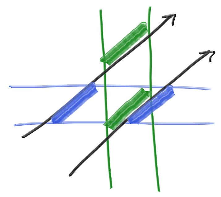
劣線形性を達成するには、包含立体の階層を考える必要がある。例えばオブジェクトの集合を二つ (赤と青) に分け、その上で二つの集合それぞれの包含立体 (直方体) を考える。このとき次の図のような状況となる:

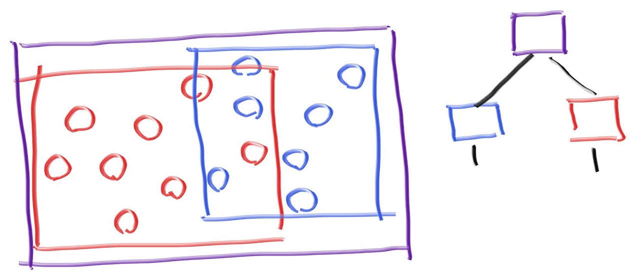
紫の包含立体には青と赤の包含立体が含まれるが、この二つは重なり得る。また青と赤の包含立体は両方とも紫の中にあるだけで、順序付いていない。図にある木では青を右の子として、赤を左の子として書いているが、この方向に意味は無い。この包含立体階層を使うコードは次のようになる:

if (紫と交わる)
  hit0 = 青に含まれるオブジェクトと交わる
  hit1 = 赤に含まれるオブジェクトと交わる
  if (hit0 or hit1)
    return (true, 近い方の交点の情報)
return false

軸平行包含直方体

以上のアイデアを実装するには、包含立体とレイの衝突判定とオブジェクトの良い分割処理が必要になる (悪い分割も存在する)。包含立体とレイの衝突判定は高速である必要があり、さらに包含立体は小さくなければならない。現実で扱う多くのモデルでは辺が軸に平行な直方体が包含立体として他の選択肢よりも優れている。ただし変わったモデルを扱うときには他の選択肢もあることを思い出せるようにしておくべきである。

正確に「辺が軸に平行な包含直角平行六面体」と呼んだのでは長すぎるので、これからは軸平行包含直方体 (axis-aligned bounding box, AABB) と呼ぶ。レイと AABB の衝突判定にはどんな方法を使っても構わない。また知りたいのは衝突するかどうかだけであり、描画するオブジェクトとの衝突判定のように衝突点やそこでの法線といった情報は必要ない。

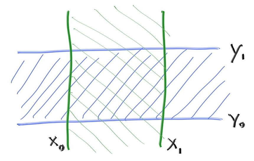
レイと AABB の衝突判定には「スラブ」を使った方法が使われることが多い³。この方法は \(n\) 次元の AABB が \(n\) 個の軸に平行な区間の和集合として表せるという観察を利用する。区間とは二つの端点に挟まれた点の集合であり、例えば「\(3 \lt x \lt 5\) を満たす \(x\)」あるいは「\((3, 6)\)に含まれる \(x\)」は区間を定義する。二次元では、\(x\) の区間と \(y\) の区間が 2D の AABB (長方形) を構成する:

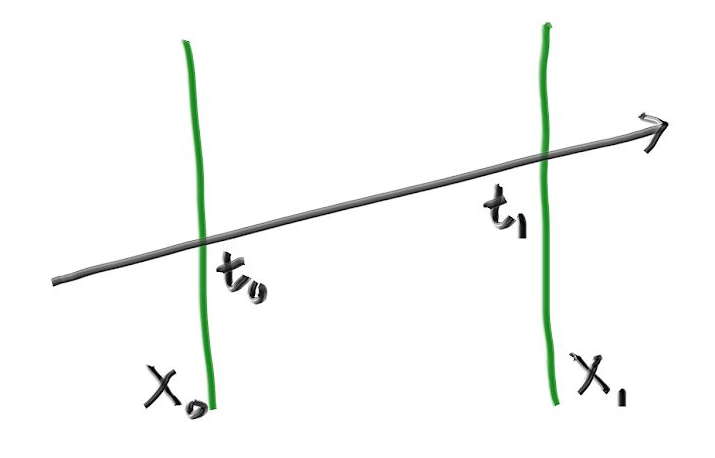
レイと区間の衝突を判定するには、まずレイが区間の境界 (スラブ) と交わるかを調べる。二次元の例であれば、レイがスラブと交わるときのレイのパラメータは \(t_{0}\) および \(t_{1}\) と表せる (スラブと平行なレイでは \(t_{0}\) と \(t_{1}\) は定義されない)。

三次元では区間の境界が平面になり、その方程式は \(x = x_{0}\) および \(x = x_{1}\) と表せる (\(x\) の区間の場合)。この平面とレイはどこで交わるだろうか？レイは実数 \(t\) を受け取って位置 \(\textbf{P}(t)\) を返す関数 \[ \mathbf{P}(t) = \mathbf{A} + t \mathbf{b} \] と考えることができ、この等式は \(x\), \(y\), \(z\) 座標のそれぞれで成り立つ。例えば \(x\) 座標では \(x(t) = A_{x} + t b_{x}\) となる。よってこのレイが平面 \(x = x_{0}\) と交わるときの \(t\) で次の等式が成り立つ: \[ x_0 = A_x + t_0 b_x \] したがって交点における \(t = t_{0}\) で \[ t_0 = \frac{x_0 - A_x}{b_x} \] だと分かる。\(x_{1}\) についても同様に \[ t_1 = \frac{x_1 - A_x}{b_x} \] を得る。この一次元の結果を使って衝突を判定するときに鍵となるのが、座標ごとの \(t\) の区間が重なるなら例と AABB が衝突するという事実である。例えば次の二次元の例では、レイと長方形が衝突するときに限って緑と青の区間が重なる:

AABB を使ったレイの衝突判定

次の疑似コードはレイがスラブを通る \(t\) の値を求め、座標ごとの \(t\) の区間が重なるかを判定する:

compute (tx0, tx1)
compute (ty0, ty1)
return overlap?( (tx0, tx1), (ty0, ty1))

これは素晴らしく簡単である。この方法は三次元でも同じように使えるというのが、多くの人々から AABB が選ばれる理由となっている:

compute (tx0, tx1)
compute (ty0, ty1)
compute (tz0, tz1)
return overlap?( (tx0, tx1), (ty0, ty1), (tz0, tz1))

このスラブを使った方法にはいくつか注意点があるから、一見したほどには美しくないかもしれない。第一に、\(x\) 軸負方向に進むレイに対して上記の方法で区間 \(t_{x_{0}}, t_{x_{1}}\) を計算すると、\((7, 3)\) のように反転した区間が手に入る可能性がある。第二に、除算で無限大が生じる可能性がある。さらに、レイの始点がスラブの境界上にあると計算結果に NaN が生じる可能性がある。様々なレイトレーサーは様々な方法で AABB に関する問題に対処している (さらに SIMD などのベクトル化から生まれる問題もある。ベクトル化を使ってさらなる高速化を行いたいなら、Ingo Wald による論文が最初に読むものとして優れている)。今の私たちのプログラムでは、この部分はそれなりに速くしておけば大きなボトルネックになることはない。というわけで、できるだけ単純に実装しよう。そうするのが最も高速な場合もよくあるのだから！まず区間を表す式に注目する: \[ \begin{aligned} t_{x_{0}} & = \frac{x_0 - A_x}{b_x} \\ t_{x_{1}} & = \frac{x_1 - A_x}{b_x} \end{aligned} \] ここで問題なのが、何の変哲もない普通のレイでも \(b_{x} = 0\) となって \(0\) 除算が発生することがあり得る点である。そういったレイはスラブの外側にあるかもしれないし、内側にあるかもしれない。また IEEE 浮動小数点数の \(0\) には \(\pm\) の符号がある。ただここで、\(b_{x} = 0\) となるレイが \(x_{0}\) から \(x_{1}\) の間にないなら \(t_{x_{0}}\) と \(t_{x_{1}}\) は両方とも \(\infty\) となるか両方とも \(-\infty\) のなるかのどちらかであるという事実が利用できる。つまり \(\min\) と \(\max\) を使って \(t_{x_{0}}\) と \(t_{x_{1}}\) を求めれば、どんな場合にも正しい区間が計算される: \[ \begin{aligned} t_{x_{0}} & = \min \left( \frac{x_0 - A_x}{b_x}, \frac{x_1 - A_x}{b_x} \right) \\ t_{x_{1}} & = \max \left( \frac{x_0 - A_x}{b_x}, \frac{x_1 - A_x}{b_x} \right) \end{aligned} \]

もう一つ問題なのが \(b_{x} = 0\) かつ「\(x_{0} - A_{x} = 0\) または \(x_{1} - A_{x} = 0\)」となるときである。このとき NaN となってしまう。ただこの場合にはレイが交わるとしても交わらないとしても大きな問題はない。後でもう一度触れる。

続いて重なりを判定する関数を考えよう。区間が反転していない (一つ目の値が二つ目の値より小さい) として、区間が重なるとき true を返すとする。区間 \(d, D\) と \(e, E\) が重なるかを調べ、重なる場合には共通する区間 \(f, F\) を計算する関数は次のように書ける:

bool overlap(d, D, e, E, f, F)
  f = max(d, e)
  F = min(D, E)
  return (f < F)

入力に NaN が含まれるとき、この関数は false を返す。つまり AABB と水平に近い角度で衝突するレイを扱うには、AABB を本来よりも少しだけ大きく取る必要がある (レイトレーサーではどんな可能性もいずれ起こるので、こうしなければならない)。三つの次元をループで扱うようにして、さらに区間 \(t_{\text{min}}, t_{\text{max}}\) を関数の引数として渡すようにすれば次のコードを得る:

#include "rtweekend.h"

class aabb {
public:
  aabb() {}
  aabb(const point3& a, const point3& b) { _min = a; _max = b;}

  point3 min() const {return _min; }
  point3 max() const {return _max; }

  bool hit(const ray& r, double tmin, double tmax) const {
    for (int a = 0; a < 3; a++) {
      auto t0 = fmin((_min[a] - r.origin()[a]) / r.direction()[a],
                     (_max[a] - r.origin()[a]) / r.direction()[a]);
      auto t1 = fmax((_min[a] - r.origin()[a]) / r.direction()[a],
                     (_max[a] - r.origin()[a]) / r.direction()[a]);
      tmin = fmax(t0, tmin);
      tmax = fmin(t1, tmax);
      if (tmax <= tmin)
        return false;
    }
    return true;
  }

  point3 _min;
  point3 _max;
};

リスト 2.8 [aabb.h] aabb クラス

AABB の衝突判定の最適化

この衝突判定法をレビューしたピクサーの Anrew Kensler は実験を行い、次のコードを提案した。これはコンパイラに関わらず非常に高速なので、私はこちらを使うようにしている:

inline bool aabb::hit(const ray& r, double tmin, double tmax) const {
  for (int a = 0; a < 3; a++) {
    auto invD = 1.0f / r.direction()[a];
    auto t0 = (min()[a] - r.origin()[a]) * invD;
    auto t1 = (max()[a] - r.origin()[a]) * invD;
    if (invD < 0.0f)
      std::swap(t0, t1);
    tmin = t0 > tmin ? t0 : tmin;
    tmax = t1 < tmax ? t1 : tmax;
    if (tmax <= tmin)
      return false;
  }
  return true;
}

リスト 2.9 [aabb.h] AABB の衝突判定 (最適化後)

AABB の構築

続いて hittable 全体に対する AABB を計算する関数が必要になる。計算するのはシーンに含まれる全てのプリミティブに関する AABB の階層であり、球などの個々のプリミティブが葉となる。無限に広がる平面のように AABB を持たないプリミティブもあるので、この関数は AABB が構築できたかを表す bool 値を返す。また移動するオブジェクトに関しては、その AABB が time0 から time1 まで全ての時刻におけるオブジェクトを含むことになる。

class hittable {
public:
  virtual bool hit(
    const ray& r, double t_min, double t_max, hit_record& rec
  ) const = 0;
  virtual bool bounding_box(double t0, double t1, aabb& output_box) const = 0;
};

リスト 2.10 [hittable.h] hittable クラスに AABB を追加する

球の bounding_box 関数は簡単に書ける:

bool sphere::bounding_box(double t0, double t1, aabb& output_box) const {
  output_box = aabb(center - vec3(radius, radius, radius),
                    center + vec3(radius, radius, radius));
  return true;
}

リスト 2.11 [sphere.h] sphere::bounding_box 関数

moving_sphere ではまず \(t_{0}\) における AABB と \(t_{1}\) における AABB 計算し、二つの AABB を含む AABB をさらに計算すればよい:

bool moving_sphere::bounding_box(double t0, double t1, aabb& output_box) const {
  aabb box0(center(t0) - vec3(radius, radius, radius),
            center(t0) + vec3(radius, radius, radius));
  aabb box1(center(t1) - vec3(radius, radius, radius),
            center(t1) + vec3(radius, radius, radius));
  output_box = surrounding_box(box0, box1);
  return true;
}

リスト 2.12 [moving_sphere.h] moving_sphere::bounding_box 関数

二つの AABB の AABB を計算する surrouding_box 関数は次のように書ける:

aabb surrounding_box(aabb box0, aabb box1) {
  point3 small(fmin(box0.min().x(), box1.min().x()),
               fmin(box0.min().y(), box1.min().y()),
               fmin(box0.min().z(), box1.min().z()));

  point3 big(fmax(box0.max().x(), box1.max().x()),
             fmax(box0.max().y(), box1.max().y()),
             fmax(box0.max().z(), box1.max().z()));

  return aabb(small,big);
}

リスト 2.13 [aabb.h] AABB の AABB

オブジェクトリストの AABB の計算

リストの AABB は作成時に計算することもできるし、bounding_box を呼び出したときその場で計算することもできる。通常 bounding_box は BVH を構築するときに一度だけ呼ばれるので、私はその場で AABB を計算させる方法を取る:

bool hittable_list::bounding_box(double t0, double t1, aabb& output_box) const {
  if (objects.empty()) return false;

  aabb temp_box;
  bool first_box = true;

  for (const auto& object : objects) {
    if (!object->bounding_box(t0, t1, temp_box)) return false;
    output_box = first_box ? temp_box : surrounding_box(output_box, temp_box);
    first_box = false;
  }

  return true;
}

リスト 2.14 [hittable_list.h] hittable_list::bounding_box 関数

BVH を表すクラス

BVH は ── hittable のリストと同様に── hittable となる。BVH は他の hittable を保持するコンテナに過ぎないが、「このレイと交わるか？」という質問には答えることができる。BVH を設計するときの選択肢として、木とノードを表すクラスをそれぞれ作る方法と、ノードを表すクラスだけを作って木をノードとして表す方法がある。私は可能な限りクラスを一つだけ使った設計を使うようにしている。BVH を表すクラスを示す:

class bvh_node : public hittable {
public:
  bvh_node();

  bvh_node(hittable_list& list, double time0, double time1)
    : bvh_node(list.objects, 0, list.objects.size(), time0, time1)
  {}

  bvh_node(
    std::vector<shared_ptr<hittable>>& objects,
    size_t start, size_t end, double time0, double time1);

  virtual bool hit(
    const ray& r, double tmin, double tmax, hit_record& rec
  ) const;
  virtual bool bounding_box(double t0, double t1, aabb& output_box) const;

public:
  shared_ptr<hittable> left;
  shared_ptr<hittable> right;
  aabb box;
};

bool bvh_node::bounding_box(double t0, double t1, aabb& output_box) const {
  output_box = box;
  return true;
}

リスト 2.15 [bvh.h] 包含立体階層 (BVH)

子へのポインタが一般的な hittable となっている点に注目してほしい。子は bvh_node にも sphere にも他の hittable にもなれる。

bvh_node の hit 関数は非常に簡単である: そのノードが持つ AABB と交わるか調べ、もし交わるなら子に詳細を調べさせればよい:

bool bvh_node::hit(
  const ray& r, double t_min, double t_max, hit_record& rec
) const {
  if (!box.hit(r, t_min, t_max))
    return false;

  bool hit_left = left->hit(r, t_min, t_max, rec);
  bool hit_right = right->hit(r, t_min, hit_left ? rec.t : t_max, rec);

  return hit_left || hit_right;
}

リスト 2.16 [bvh.h] bvh_node::hit 関数

BVH の分割

効率化のためのデータ構造で最も複雑になるのはその構築であり、BVH も例外ではない。BVH の構築は bvh_node のコンストラクタで行う。ただ BVH で素晴らしいのが、bvh_node に渡されるオブジェクトの集合を二つに分けさえすれば hit 関数が正しく動く点である。もちろん二つの子の AABB が親の AABB より小さくなる分割が望ましいが、分割の質が関係するのは実行速度だけで正しさは関係しない。ここでは単純さと効率の妥協点となるアルゴリズムとして、各ノードで一つの軸に沿ってオブジェクトを分割する方法を採用する。つまり

ランダムに軸を選ぶ。
プリミティブを (std::sort で) ソートする
オブジェクトを半分ずつ子に入れ、子を再帰的に分割する。

という操作を行う。

受け取ったリストが持つ要素が二つだけなら、左および右の子に一つずつ要素を設定して再帰を終える。走査アルゴリズムは高速である必要があり、ヌルポインタをチェックしている暇はないので、要素が一つの場合には二つの子に同じオブジェクトを入れる。要素が三つのときを明示的に処理して再帰をなくしたとしてもあまり高速にならないだろう。いずれにせよこのメソッドは後で高速化する可能性が高い。

#include <algorithm>
...

inline int random_int(int min, int max) {
  // {min, min+1, ..., max} から整数をランダムに返す
  return min + rand() % (max - min + 1);
}

bvh_node::bvh_node(
  std::vector<shared_ptr<hittable>>& objects,
  size_t start, size_t end, double time0, double time1
) {
  int axis = random_int(0,2);
  auto comparator = (axis == 0) ? box_x_compare
                  : (axis == 1) ? box_y_compare
                  : box_z_compare;

  size_t object_span = end - start;

  if (object_span == 1) {
    left = right = objects[start];
  } else if (object_span == 2) {
    if (comparator(objects[start], objects[start+1])) {
      left = objects[start];
      right = objects[start+1];
    } else {
      left = objects[start+1];
      right = objects[start];
    }
  } else {
    std::sort(objects.begin() + start, objects.begin() + end, comparator);

    auto mid = start + object_span/2;
    left = make_shared<bvh_node>(objects, start, mid, time0, time1);
    right = make_shared<bvh_node>(objects, mid, end, time0, time1);
  }

  aabb box_left, box_right;

  if (  !left->bounding_box (time0, time1, box_left)
     || !right->bounding_box(time0, time1, box_right))
    std::cerr << "No bounding box in bvh_node constructor.\n";

  box = surrounding_box(box_left, box_right);
}

リスト 2.17 [bvh.h] BVH の構築

AABB の存在を確認しているのは、無限に広がる平面のように AABB が存在しないオブジェクトが存在するためである。今の段階ではそういったオブジェクトを実装していないから、明示的に追加するまでこのエラーは起こらない。

AABB の比較関数

次に std::sort() が使う AABB の比較関数を実装する必要がある。二つの AABB を引数で表される軸で比較する一般的な関数を作れば、軸に関する比較はこの一般的な関数を使って書ける:

inline bool box_compare(
  const shared_ptr<hittable> a, const shared_ptr<hittable> b, int axis
) {
  aabb box_a;
  aabb box_b;

  if (!a->bounding_box(0,0, box_a) || !b->bounding_box(0,0, box_b))
    std::cerr << "No bounding box in bvh_node constructor.\n";

  return box_a.min().e[axis] < box_b.min().e[axis];
}


bool box_x_compare (
  const shared_ptr<hittable> a, const shared_ptr<hittable> b
) {
  return box_compare(a, b, 0);
}

bool box_y_compare (
  const shared_ptr<hittable> a, const shared_ptr<hittable> b
) {
  return box_compare(a, b, 1);
}

bool box_z_compare (
  const shared_ptr<hittable> a, const shared_ptr<hittable> b
) {
  return box_compare(a, b, 2);
}

リスト 2.18 [bvh.h] AABB の比較関数

## ソリッドテクスチャ

グラフィックスにおける「テクスチャ」は物体表面の色を何らかの規則に従ってプロシージャルに生成する関数を表す。この規則には画像を合成するコードや既存の画像のルックアップが関係し、両方が含まれる場合もある。この節ではまずこれまでのプログラムに含まれる全ての色をテクスチャに変更する。定数の RGB 色とテクスチャを異なるクラスで管理するプログラムも多いので、別の方法を取っても構わない。ただ任意の色をテクスチャとして扱えるのは美しいので、私はこのアーキテクチャを大いに気に入っている。

最初のテクスチャクラス: 定数テクスチャ

#include "rtweekend.h"

class texture {
public:
  virtual ~texture() {}
  virtual color value(double u, double v, const point3& p) const = 0;
};

class solid_color : public texture {
public:
  solid_color() {}
  solid_color(color c) : color_value(c) {}

  solid_color(double red, double green, double blue)
    : solid_color(color(red,green,blue)) {}

  virtual color value(double u, double v, const vec3& p) const {
    return color_value;
  }

private:
  color color_value;
};

リスト 2.19 [texture.h] texture クラス

レイとオブジェクトの交点のテクスチャ座標 \((u, v)\) を保存するよう hit_record 構造体を変更する必要がある:

struct hit_record {
  vec3 p;
  vec3 normal;
  shared_ptr<material> mat_ptr;
  double t;
  double u;
  double v;
  bool front_face;
  ...

リスト 2.20 [hittable.h] hit_record にテクスチャ座標を追加する

続いて hittable を継承するクラスでテクスチャ座標 \((u, v)\) の計算を行う。

球のテクスチャ座標

球では緯度と経度からなる球面座標を使ってテクスチャ座標を計算する。球上の点の球面座標 \((\theta, \phi)\) が分かれば、\(\theta\) と \(\phi\) に定数を乗じることでテクスチャ座標が求まる。\(\theta\) が極から下向きに測った角度で \(\phi\) が極を通る軸周りの角度なら、二つの角度から \([0,1]\) への変換は \[ u = \frac{\phi}{2\pi}, \quad v = \frac{\theta}{\pi} \] となる。

交点に対応する \(\theta\) と \(\phi\) の計算では、単位球上の点に対する球面座標の公式を利用する: \[ \begin{aligned} x & = \cos\phi \cos\theta \\ y & = \sin\phi \cos\theta \\ z & = \sin\theta \end{aligned} \] これを逆にすればよい。<cmath> にはサインとコサインの値から角度を求める素晴らしい関数 atan2() があるから、これに \(x\) と \(y\) を渡せば \[ \phi = \operatorname{atan2}(y, x) \] となる (\(\cos\theta\) は打ち消される)。\(\operatorname{atan2}\) は \(-\pi\) から \(\pi\) の値を取るので、この後に少し調整が必要になる。また \(\theta\) は簡単に求まる: \[ \theta = \operatorname{asin}(z) \] \(\operatorname{asin}\) は \(-\pi/2\) から \(\pi/2\) の値を返す。

sphere::hit 関数での \((u, v)\) 座標の計算はユーティリティ関数を使って行う。この関数が受け取るのは単位球上の点であり、呼び出し側では次のようにする:

get_sphere_uv((rec.p-center)/radius, rec.u, rec.v);

リスト 2.21 [sphere.h] 交点の UV 座標を求める

ユーティリティ関数の本体を示す:

void get_sphere_uv(const vec3& p, double& u, double& v) {
  auto phi = atan2(p.z(), p.x());
  auto theta = asin(p.y());
  u = 1-(phi + pi) / (2*pi);
  v = (theta + pi/2) / pi;
}

リスト 2.22 [sphere.h] get_sphere_uv 関数

後はマテリアルクラスの色を保持する変数 const color& a をテクスチャへのポインタ shared_ptr<texture> a に変更すれば、テクスチャを使うマテリアルが完成する:

class lambertian : public material {
public:
  lambertian(shared_ptr<texture> a) : albedo(a) {}

  virtual bool scatter(
    const ray& r_in, const hit_record& rec, color& attenuation, ray& scattered
  ) const {
    vec3 scatter_direction = rec.normal + random_unit_vector();
    scattered = ray(rec.p, scatter_direction, r_in.time());
    attenuation = albedo->value(rec.u, rec.v, rec.p);
    return true;
  }

public:
  shared_ptr<texture> albedo;
};

リスト 2.23 [material.h] テクスチャを使ったランバーティアンマテリアル

これまでのコードには次のような部分があった:

  ...make_shared<lambertian>(color(0.5, 0.5, 0.5))

リスト 2.24 [main.cc] color を使ったランバーティアンマテリアル

この color(...) を make_shared<solid_color>(...) に入れ替えよう:

  ...make_shared<lambertian>(make_shared<solid_color>(0.5, 0.5, 0.5))

リスト 2.25 [main.cc] テクスチャを使ったランバーティアンマテリアル

main.cc の random_scene() にある三つのランバーティアンを更新すれば、以前と同じ画像をレンダリングできるようになる。

縞模様テクスチャ

サインとコサインの符号が周期的に反転することを利用すれば縞模様 (チェッカー) テクスチャを作ることができる。また各座標に三角関数を適用して積を取れば、その積の符号は三次元の縞模様となる。

class checker_texture : public texture {
public:
  checker_texture() {}
  checker_texture(shared_ptr<texture> t0, shared_ptr<texture> t1)
  : even(t0), odd(t1) {}

  virtual color value(double u, double v, const point3& p) const {
    auto sines = sin(10*p.x())*sin(10*p.y())*sin(10*p.z());
    if (sines < 0)
      return odd->value(u, v, p);
    else
      return even->value(u, v, p);
  }

public:
  shared_ptr<texture> even;
  shared_ptr<texture> odd;
};

リスト 2.26 [texture.h] 縞模様テクスチャ

この縞模様の偶奇に対応するテクスチャには定数テクスチャだけではなく任意のプロシージャルなテクスチャを設定できる。ここには Pat Hanrahan によって 1980 年代に提案されたシェーダーネットワークの考え方が生きている。

random_scene() 関数の地面代わりの球にこのテクスチャを追加しよう:

auto checker = make_shared<checker_texture>(
  make_shared<solid_color>(0.2, 0.3, 0.1),
  make_shared<solid_color>(0.9, 0.9, 0.9)
);

world.add(
  make_shared<sphere>(point3(0,-1000,0), 1000, make_shared<lambertian>(checker))
);

リスト 2.27 [main.cc] 縞模様テクスチャを使う

次の画像が得られる:

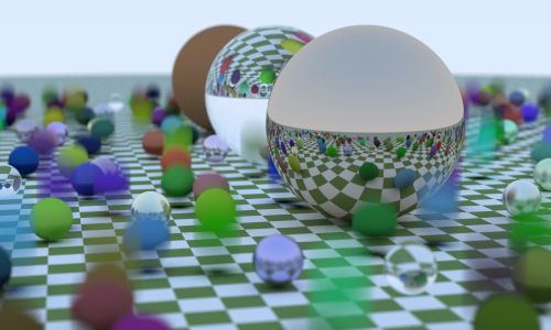
縞模様テクスチャを使ったシーンのレンダリング

新しくシーンを追加する:

hittable_list two_spheres() {
  hittable_list objects;

  auto checker = make_shared<checker_texture>(
    make_shared<solid_color>(0.2, 0.3, 0.1),
    make_shared<solid_color>(0.9, 0.9, 0.9)
  );

  objects.add(
    make_shared<sphere>(point3(0,-10, 0), 10, make_shared<lambertian>(checker))
  );
  objects.add(
    make_shared<sphere>(point3(0, 10, 0), 10, make_shared<lambertian>(checker))
  );

  return objects;
}

リスト 2.28 [main.cc] 縞模様の球が二つあるシーン

カメラは次の位置に配置する:

const auto aspect_ratio = double(image_width) / image_height;
...
point3 lookfrom(13,2,3);
point3 lookat(0,0,0);
vec3 vup(0,1,0);
auto dist_to_focus = 10.0;
auto aperture = 0.0;

camera cam(
  lookfrom, lookat, vup, 20, aspect_ratio, aperture, dist_to_focus, 0.0, 1.0
);

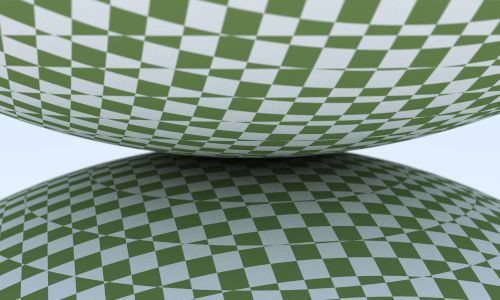
リスト 2.29 [main.cc] 視点に関するパラメータ

次の画像が得られる:

パーリンノイズ

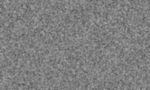
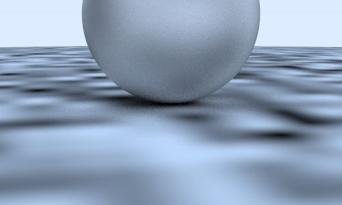
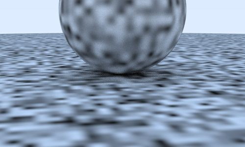
クールな見た目のソリッドテクスチャはパーリンノイズ (Perlin noise) の一種を使って作られることが多い。考案者のケン・パーリン (Ken Perlin) の名前が付いたこのノイズを使ったテクスチャは、次のホワイトノイズのようにはならない:

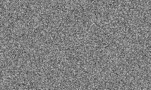
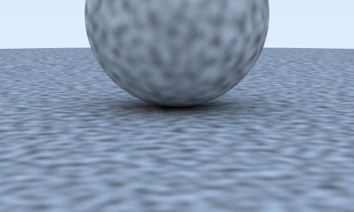
パーリンノイズによって計算されるテクスチャは、次のぼかしたホワイトノイズに似ている:

パーリンノイズで重要なのが、反復できることである。パーリンノイズは三次元の点を入力として受け取り、乱数らしき値を返す。同じ入力に対する出力はいつでも同じであり、近い点に対しては近い値が出力される。さらにパーリンノイズに関してもう一つ重要なのが、単純で高速なことだ。そのためこのノイズはハックとして実装されることが多い。ここでは Andrew Kensler の説明に沿ってインクリメンタルに実装していく。

乱数のブロック

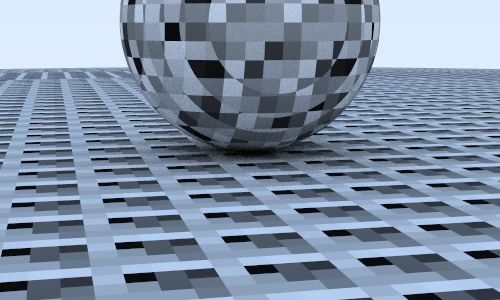
ノイズの生成方法として、適当な大きさの乱数を三次元配列に格納し、それを一つのブロックとして空間内に敷き詰めるという方法がまず考えられる。こうして得られるのは角ばったテクスチャであり、パターンも明らかである:

乱数のブロックを敷き詰める代わりに、ハッシュのような処理を使って添え字をかき混ぜてみよう。この処理には少しコードが必要になる:

class perlin {
public:
  perlin() {
    ranfloat = new double[point_count];
    for (int i = 0; i < point_count; ++i) {
      ranfloat[i] = random_double();
    }

    perm_x = perlin_generate_perm();
    perm_y = perlin_generate_perm();
    perm_z = perlin_generate_perm();
  }

  ~perlin() {
    delete[] ranfloat;
    delete[] perm_x;
    delete[] perm_y;
    delete[] perm_z;
  }

  double noise(const point3& p) const {
    auto i = static_cast<int>(4*p.x()) & 255;
    auto j = static_cast<int>(4*p.y()) & 255;
    auto k = static_cast<int>(4*p.z()) & 255;

    return ranfloat[perm_x[i] ^ perm_y[j] ^ perm_z[k]];
  }

private:
  static const int point_count = 256;
  double* ranfloat;
  int* perm_x;
  int* perm_y;
  int* perm_z;

  static int* perlin_generate_perm() {
    auto p = new int[point_count];

    for (int i = 0; i < perlin::point_count; i++)
      p[i] = i;

    permute(p, point_count);

    return p;
  }

  static void permute(int* p, int n) {
    for (int i = n-1; i > 0; i--) {
      int target = random_int(0, i);
      int tmp = p[i];
      p[i] = p[target];
      p[target] = tmp;
    }
  }
};

リスト 2.30 [perline.h] パーリンノイズを表すクラス

このクラスを使って \(0\) から \(1\) までの float を生成し、それを使ってグレーの色を作成するテクスチャ noise_texture を実装する:

#include "perlin.h"

class noise_texture : public texture {
public:
  noise_texture() {}

  virtual color value(double u, double v, const point3& p) const {
    return color(1,1,1) * noise.noise(p);
  }

public:
  perlin noise;
};

リスト 2.31 [texture.h] ノイズテクスチャ

このテクスチャを球に割り当てよう:

hittable_list two_perlin_spheres() {
  hittable_list objects;

  auto pertext = make_shared<noise_texture>();
  objects.add(make_shared<sphere>(
    point3(0,-1000,0), 1000, make_shared<lambertian>(pertext))
  );
  objects.add(make_shared<sphere>(
    point3(0, 2, 0), 2, make_shared<lambertian>(pertext))
  );

  return objects;
}

リスト 2.32 [main.cc] パーリンテクスチャを持つ球を二つ配置したシーン

カメラは前と同じとする:

const auto aspect_ratio = double(image_width) / image_height;
...
point3 lookfrom(13,2,3);
point3 lookat(0,0,0);
vec3 vup(0,1,0);
auto dist_to_focus = 10.0;
auto aperture = 0.0;

camera cam(
  lookfrom, lookat, vup, 20, aspect_ratio, aperture, dist_to_focus, 0.0, 1.0
);

リスト 2.33 [main.cc] 視点のパラメータ

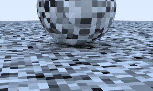
レンダリング結果からは、期待通りハッシュによってテクスチャがかき混ざったことが分かる:

ノイズのスムージング

線形補間を行えば値をスムーズにできる:

inline double trilinear_interp(
  double c[2][2][2], double u, double v, double w
) {
  auto accum = 0.0;
  for (int i=0; i < 2; i++)
    for (int j=0; j < 2; j++)
      for (int k=0; k < 2; k++)
        accum += (i*u + (1-i)*(1-u))*
                 (j*v + (1-j)*(1-v))*
                 (k*w + (1-k)*(1-w))*c[i][j][k];

  return accum;
}

class perlin {
public:
  ...
  double noise(point3 vec3& p) const {
    auto u = p.x() - floor(p.x());
    auto v = p.y() - floor(p.y());
    auto w = p.z() - floor(p.z());
    int i = floor(p.x());
    int j = floor(p.y());
    int k = floor(p.z());
    double c[2][2][2];

    for (int di=0; di < 2; di++)
      for (int dj=0; dj < 2; dj++)
        for (int dk=0; dk < 2; dk++)
          c[di][dj][dk] = ranfloat[
            perm_x[(i+di) & 255] ^
            perm_y[(j+dj) & 255] ^
            perm_z[(k+dk) & 255]
          ];

    return trilinear_interp(c, u, v, w);
  }
  ...
}

リスト 2.34 [perlin.h] 三次元線形補間を使ったパーリンノイズ

次の画像が得られる:

エルミート補間によるノイズの改善

線形補間により見た目は改善されたが、まだ元のグリッドが残って見える。色の線形補間で起こるマッハバンド (Mach band) と呼ばれる錯覚が原因の一つである。ここでよく使われるのが、三次エルミート補間を使って値の変化を滑らかにするというテクニックだ:

class perlin {
public:
  ...
  double noise(const point3& p) const {
    auto u = p.x() - floor(p.x());
    auto v = p.y() - floor(p.y());
    auto w = p.z() - floor(p.z());

    u = u*u*(3-2*u);
    v = v*v*(3-2*v);
    w = w*w*(3-2*w);

    int i = floor(p.x());
    int j = floor(p.y());
    int k = floor(p.z());
    ...

リスト 2.35 [perlin.h] パーリンノイズを滑らかにする

さらにスムーズな画像 (図 2.13) が得られる。

周波数の調整

このテクスチャは周波数が低すぎる (値の変化が遅すぎる) ように見える。入力点をスケールすれば、ノイズがもっと速く変化させることができる:

class noise_texture : public texture {
public:
  noise_texture() {}
  noise_texture(double sc) : scale(sc) {}

  virtual color value(double u, double v, const point3& p) const {
    return color(1,1,1) * noise.noise(scale * p);
  }

public:
  perlin noise;
  double scale;
};

リスト 2.36 [perlin.h] 周波数を追加した noise_texture

scale を 5 とすれば図 2.14 を得る。

格子点にランダムなベクトルを配置する

これでもまだ角張って見える。模様の最大値と最小値が常に \(x\), \(y\), \(z\) が整数の部分にあることが理由として考えられる。Ken Perlin が考案した非常に賢いトリックは、格子点に (float ではなく) ランダムな単位ベクトルを割り当てて、内積を使って最大値と最小値を格子点から動かすというものである。格子点に割り当てるベクトルはパターンが明らかでなければ完全にランダムでなくても構わないので、ここでは前もって計算したベクトルを用いる:

class perlin {
public:
  perlin() {
    ranvec = new vec3[point_count];

    for (int i = 0; i < point_count; ++i) {
      ranvec[i] = unit_vector(vec3::random(-1,1));
    }

    perm_x = perlin_generate_perm();
    perm_y = perlin_generate_perm();
    perm_z = perlin_generate_perm();
  }

  ~perlin() {
    delete[] ranvec;
    delete[] perm_x;
    delete[] perm_y;
    delete[] perm_z;
  }
...
private:
  vec3* ranvec;
  int* perm_x;
  int* perm_y;
  int* perm_z;
  ...
}

リスト 2.37 [perlin.h] ランダムな単位長の変位を追加した perlin

perlin::noise() は次のようになる:

class perlin {
public:
  ...
  double noise(const point3& p) const {
    auto u = p.x() - floor(p.x());
    auto v = p.y() - floor(p.y());
    auto w = p.z() - floor(p.z());
    int i = floor(p.x());
    int j = floor(p.y());
    int k = floor(p.z());
    vec3 c[2][2][2];

    for (int di=0; di < 2; di++)
      for (int dj=0; dj < 2; dj++)
        for (int dk=0; dk < 2; dk++)
          c[di][dj][dk] = ranvec[
            perm_x[(i+di) & 255] ^
            perm_y[(j+dj) & 255] ^
            perm_z[(k+dk) & 255]
          ];

    return perlin_interp(c, u, v, w);
  }
  ...
}

リスト 2.38 [perlin.h] ランダムなベクトルを使う perlin::noise()

補間 perlin_interp() はさらに複雑になる:

class perlin {
...
private:
  ...
  inline double perlin_interp(vec3 c[2][2][2], double u, double v, double w) {
    auto uu = u*u*(3-2*u);
    auto vv = v*v*(3-2*v);
    auto ww = w*w*(3-2*w);
    auto accum = 0.0;

    for (int i=0; i < 2; i++)
      for (int j=0; j < 2; j++)
        for (int k=0; k < 2; k++) {
          vec3 weight_v(u-i, v-j, w-k);
          accum += (i*uu + (1-i)*(1-uu)) *
                   (j*vv + (1-j)*(1-vv)) *
                   (k*ww + (1-k)*(1-ww)) * dot(c[i][j][k], weight_v);
        }

    return accum;
  }
...
}

リスト 2.39 [perlin.h] パーリンノイズの補間関数

この補間関数の出力は負になる可能性がある。負の値がガンマ補正関数の sqrt() に渡されると NaN が発生するので、perlin_texture ではパーリンノイズからの出力を \(0\) から \(1\) に変換する:

class noise_texture : public texture {
public:
  noise_texture() {}
  noise_texture(double sc) : scale(sc) {}

  virtual color value(double u, double v, const point3& p) const {
    return color(1,1,1) * 0.5 * (1.0 + noise.noise(scale * p));
  }

public:
  perlin noise;
  double scale;
};

リスト 2.40 [perlin.h] 変更したパーリンノイズを使う noise_texture

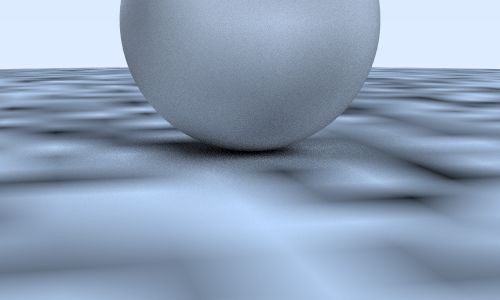
これでようやくノイズらしい見た目が得られる:

乱流ノイズ

異なる周波数のノイズを組み合わせて新しくノイズを作る方法も非常によく使われる。この方法は乱流 (turbulence) と呼ばれ、複数回呼び出したノイズの和として計算する:

class perlin {
...
public:
  ...
  double turb(const point3& p, int depth=7) const {
    auto accum = 0.0;
    auto temp_p = p;
    auto weight = 1.0;

    for (int i = 0; i < depth; i++) {
      accum += weight*noise(temp_p);
      weight *= 0.5;
      temp_p *= 2;
    }

    return fabs(accum);
  }
  ...

リスト 2.41 [perlin.h] 乱流関数

ここで使われている fabs() は絶対値を計算する関数であり、<cmath> で定義される。

乱流をそのまま使うとカモフラージュネットのような見た目が得られる:

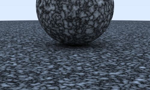
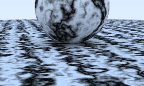
位相の調整

乱流は間接的に使われることが多い。例えばプロシージャルソリッドテクスチャにおける "hello world" である大理石模様のテクスチャは乱流を間接的に使うと作成できる。基本的な考え方は、色の濃さをサイン関数に比例させ、位相 (\(\sin x\) における \(x\)) に乱流で変化を付けて値をうねらせるというものだ。ノイズをそのまま使うコードをコメントアウトし、大理石模様のエフェクトを追加しよう:

class noise_texture : public texture {
public:
  noise_texture() {}
  noise_texture(double sc) : scale(sc) {}

  virtual color value(double u, double v, const point3& p) const {
    return color(1,1,1) * 0.5 * (1 + sin(scale*p.z() + 10*noise.turb(p)));
  }

public:
  perlin noise;
  double scale;
};

リスト 2.42 [perlin.h] パーリンノイズと乱流を使ったノイズテクスチャ

次の画像が得られる:

画像のテクスチャマッピング

前節ではレイとオブジェクトの交点 \(\textbf{P}\) を使ってソリッドテクスチャ (大理石模様) を作成した。\(\textbf{P}\) から計算される二次元の座標 \((u, v)\) を使えば、ファイルから読み込んだ画像をオブジェクトの表面に表示させることができる。

計算した \((u, v)\) を使う直接的な方法は \(u\) と \(v\) を整数 \(i\) と \(j\) に丸めて画像の \((i, j)\) にあるピクセルを読むというものだが、こうすると画像の解像度を変えるたびにコードを変える必要があるので使いにくい。そこで画像のピクセル座標ではなくテクスチャ座標を使うというグラフィックスにおいて必ず使われる慣習の一つを採用する。テクスチャ座標は画像内のピクセルの位置を割合で表す。例えば \(N_{x} \times N_{y}\) の画像の \((i, j)\) ピクセルを表すテクスチャ座標 \((u, v)\) は \[ u = \frac{i}{N_{x} - 1}, \quad v = \frac{j}{N_{y} - 1} \] となる。

画像データの読み込み

まず画像を保持するテクスチャクラスが必要になる。私がよく使う画像ユーティリティライブラリ stb_image.h をここでも使うことにする。このライブラリは画像ファイルを読み込んでデータを unsigned char の大きな配列に格納し、配列には各ピクセルの RGB を表す [0..255] が並ぶ (0 のとき黒で 255 のとき白)。次の image_texture クラスはこの画像データを使っている:

#include "rtweekend.h"
#include "rtw_stb_image.h"

#include <iostream>

class image_texture : public texture {
public:
  const static int bytes_per_pixel = 3;

  image_texture()
    : data(nullptr), width(0), height(0), bytes_per_scanline(0) {}

  image_texture(const char* filename) {
    auto components_per_pixel = bytes_per_pixel;

    data = stbi_load(
      filename, &width, &height, &components_per_pixel, components_per_pixel);

    if (!data) {
      std::cerr << "ERROR: Could not load texture image file '"
                << filename
                << "'.\n";
      width = height = 0;
    }

    bytes_per_scanline = bytes_per_pixel * width;
  }

  ~image_texture() {
    delete data;
  }

  virtual color value(double u, double v, const vec3& p) const {
    // テクスチャのデータがない場合には、そのことが分かるようにシアン色を返す。
    if (data == nullptr)
      return color(0,1,1);

    // 入力されたテクスチャ座標を [0,1] で切り捨てる。
    u = clamp(u, 0.0, 1.0);
    v = 1.0 - clamp(v, 0.0, 1.0);  // v を反転させて画像の座標系に合わせる。

    auto i = static_cast<int>(u * width);
    auto j = static_cast<int>(v * height);

    // 整数座標をさらに切り捨てる (テクスチャ座標は 1.0 になってはいけない)。
    if (i >= width)  i = width-1;
    if (j >= height) j = height-1;

    const auto color_scale = 1.0 / 255.0;
    auto pixel = data + j*bytes_per_scanline + i*bytes_per_pixel;

    return color(color_scale*pixel[0],
                 color_scale*pixel[1],
                 color_scale*pixel[2]);
  }

private:
  unsigned char *data;
  int width, height;
  int bytes_per_scanline;
};

リスト 2.43 [texture.h] image_texture クラス

格納されるデータの順序に難しいところはない。嬉しいことに、stb_image は非常に簡単に使うことができる ── main.h で rtw_stb_image.h をインクルードするだけだ:

#include "rtw_stb_image.h"

リスト 2.44 [main.cc] stb_image のインクルード

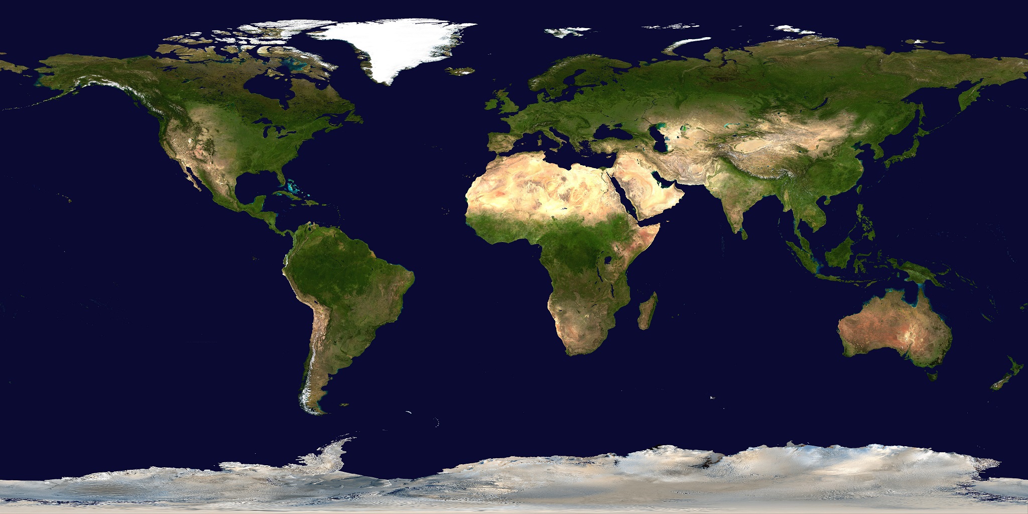
画像テクスチャを使う

適当にウェブから拾ってきた世界地図⁴を使ってみよう ──これでなくても、通常のメルカトル図法の地図なら何でもよい。

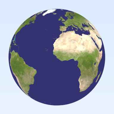
ファイルを読み込んで拡散マテリアルに割り当てるコードを示す:

hittable_list earth() {
  auto earth_texture = make_shared<image_texture>("earthmap.jpg");
  auto earth_surface = make_shared<lambertian>(earth_texture);
  auto globe = make_shared<sphere>(point3(0,0,0), 2, earth_surface);
  return hittable_list(globe);
}

リスト 2.45 [main.cc] image_texture の割り当て

全ての色をテクスチャとして扱う設計の利点が見え始めた ──lambertian マテリアルには任意のテクスチャを割り当てることができ、lambertian はテクスチャの種類を知る必要がない。

テクスチャを試すときは main.cc 内の ray_color() 関数を一時的に減衰だけを返すように変更すると分かりやすい。次の画像が得られる:

長方形とライト

ライティングはレイトレーサーの重要な要素である。初期の単純なレイトレーサーは点光源や平行光源といった抽象化された光源を使っていた。現代的なアプローチではもっと物理ベースのライトが使われるようになっており、光源は位置と大きさを持つ。この現代的な光源を実装するには、任意の通常のオブジェクトがシーン内に光を放てるよう設計を変更する必要がある。

発光マテリアル

まず光源となる発光マテリアルを作ろう。material に emitted() 関数を追加する必要がある (代わりに hit_record に変数 emitted を追加してもよい ──設計が少し変わるだけだ)。背景と同じくこの関数はレイの色を計算するだけで、反射レイは計算しない。発光する拡散マテリアルは非常に簡単に書ける:

class diffuse_light : public material  {
public:
  diffuse_light(shared_ptr<texture> a) : emit(a) {}

  virtual bool scatter(
    const ray& r_in, const hit_record& rec, color& attenuation, ray& scattered
  ) const {
    return false;
  }

  virtual color emitted(double u, double v, const point3& p) const {
    return emit->value(u, v, p);
  }

public:
  shared_ptr<texture> emit;
};

リスト 2.46 [material.h] diffuse_light クラス

発光しないマテリアルで emitted() を実装しないで済むように、基底クラスで黒を返す emitted() を実装しておく:

class material {
public:
  virtual color emitted(double u, double v, const point3& p) const {
    return color(0,0,0);
  }

  virtual bool scatter(
    const ray& r_in, const hit_record& rec, color& attenuation, ray& scattered
  ) const = 0;
};

リスト 2.47 [material.h] material クラスに emitted 関数を追加する

背景を黒くする

次に背景を完全な黒にして、シーン中のライトが全て光源から来るようにする。ray_color() 関数に背景色を表す引数 background を追加して、さらにマテリアルの emitted の値を計算に入れる:

color ray_color(
  const ray& r, const color& background, const hittable& world, int depth
) {
  hit_record rec;

  // 反射回数が一定よりも多くなったら、その時点で追跡をやめる
  if (depth <= 0)
    return color(0,0,0);

  // レイがどのオブジェクトとも交わらないなら、背景色を返す
  if (!world.hit(r, 0.001, infinity, rec))
    return background;

  ray scattered;
  color attenuation;
  color emitted = rec.mat_ptr->emitted(rec.u, rec.v, rec.p);

  if (!rec.mat_ptr->scatter(r, rec, attenuation, scattered))
    return emitted;

  return emitted
         + attenuation * ray_color(scattered, background, world, depth-1);
}
...

int main() {
  ...
  const color background(0,0,0);
  ...
        pixel_color += ray_color(r, background, world, max_depth);
  ...
}

リスト 2.48 [main.cc] 発光マテリアルに対応した ray_color() 関数

長方形オブジェクト

続いて長方形を作ろう。長方形は人工的な環境を組み立てるのに便利である。私は辺が軸に平行な長方形が実装しやすいので好きだ (後でインスタンシングを実装すれば回せるようになる)。

まず \(z\) 軸と垂直な平面を考える。\(z\) 軸と垂直な平面は \(z\) 座標の値によって \(z = k\) と定義され、その平面上の辺が軸に平行な長方形は \(x=x_{0}\), \(x=x_{1}\), \(y=y_{0}\), \(y=y_{1}\) という四本の直線で定義される。

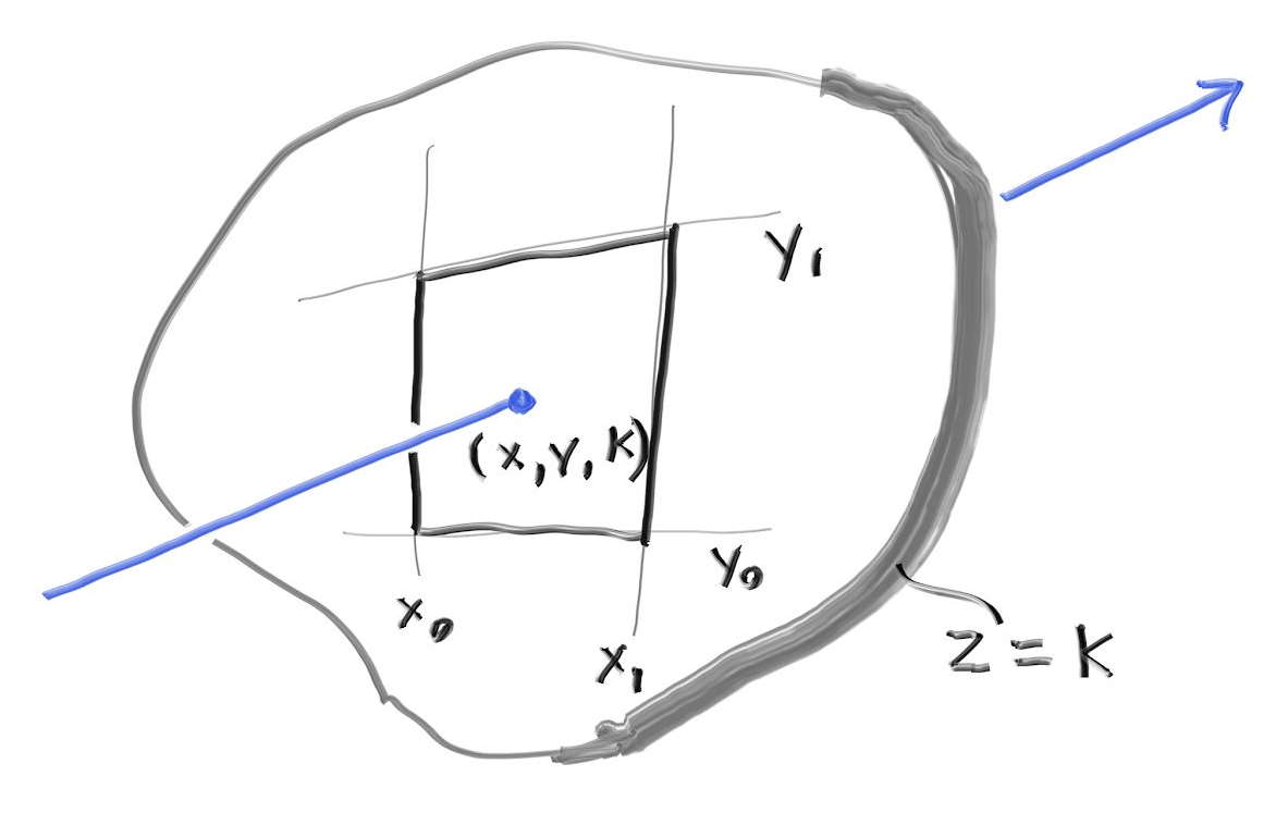
この長方形とレイが交わるかを判定するために、まずレイが平面 \(z = k\) と交わる点を求める。レイは \(\textbf{P}(t) = \textbf{A} + t \textbf{b}\) と表されるから、その \(z\) 成分は \(P_{z}(t) = A_{z} + t b_{z}\) となることは前に見た。ここから \(z = k\) における \(t\) の値が分かる: \[ t = \frac{k-A_z}{b_z} \] \(t\) が分かれば、\(\textbf{P}(t) = \textbf{A} + t \textbf{b}\) から交点の \(x\) 座標と \(y\) 座標も分かる: \[ x = A_x + t b_x ,\quad y = A_y + t b_y \]

レイが長方形と交わるのは \(x_{0} \lt x \lt x_{1}\) かつ \(y_{0} \lt y \lt y_{1}\) のときである。

今考えている長方形は辺が軸に平行だから、AABB が無限に薄くなる。AABB 階層を作るときにこれでは具合が悪いので、AABB は全ての方向に有限の大きさを持つと定め、長方形の AABB はとても薄いがゼロでない長さの辺を持つものとする。

xy_rect クラスは次のようになる:

class xy_rect: public hittable {
public:
  xy_rect() {}

  xy_rect(
    double _x0, double _x1,
    double _y0, double _y1,
    double _k,
    shared_ptr<material> mat
  ) : x0(_x0), x1(_x1),
      y0(_y0), y1(_y1),
      k(_k),
      mp(mat) {}

  virtual bool hit(const ray& r, double t0, double t1, hit_record& rec) const;

  virtual bool bounding_box(double t0, double t1, aabb& output_box) const {
    // AABB の辺の長さはゼロであってはならないので、
    // z 方向に少しだけ厚みを持たせる
    output_box = aabb(point3(x0,y0, k-0.0001), point3(x1, y1, k+0.0001));
    return true;
  }

public:
  double x0, x1, y0, y1, k;
  shared_ptr<material> mp;
};

リスト 2.49 [aarect.h] \(z\) 軸に垂直な平面を表す xy_rect クラス

hit 関数は次の通りである:

bool xy_rect::hit(const ray& r, double t0, double t1, hit_record& rec) const {
  auto t = (k-r.origin().z()) / r.direction().z();
  if (t < t0 || t > t1)
    return false;
  auto x = r.origin().x() + t*r.direction().x();
  auto y = r.origin().y() + t*r.direction().y();
  if (x < x0 || x > x1 || y < y0 || y > y1)
    return false;
  rec.u = (x-x0)/(x1-x0);
  rec.v = (y-y0)/(y1-y0);
  rec.t = t;
  auto outward_normal = vec3(0, 0, 1);
  rec.set_face_normal(r, outward_normal);
  rec.mat_ptr = mp;
  rec.p = r.at(t);
  return true;
}

リスト 2.50 [aarect.h] xy_rect::hit 関数

オブジェクトを光源にする

長方形を光源として設定する:

hittable_list simple_light() {
  hittable_list objects;

  auto pertext = make_shared<noise_texture>(4);
  objects.add(make_shared<sphere>(
    point3(0,-1000,0), 1000, make_shared<lambertian>(pertext))
  );
  objects.add(make_shared<sphere>(
    point3(0,2,0), 2, make_shared<lambertian>(pertext))
  );

  auto difflight = make_shared<diffuse_light>(make_shared<solid_color>(4,4,4));
  objects.add(make_shared<sphere>(point3(0,7,0), 2, difflight));
  objects.add(make_shared<xy_rect>(3, 5, 1, 3, -2, difflight));

  return objects;
}

リスト 2.51 [main.cc] 長方形の光源

得られるのは次の画像である:

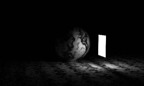
光源が \((1, 1, 1)\) よりも明るい点に注目してほしい。これによって他のオブジェクトを照らせるようになる。

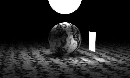
球のライトも作ればこうなる:

その他の軸に垂直な長方形

他の軸に関する長方形を追加して、有名なコーネルボックス (Cornell Box) を作ろう。

xy_rect と yz_rect はこうなる:

class xz_rect: public hittable {
public:
  xz_rect() {}

  xz_rect(
    double _x0, double _x1,
    double _z0, double _z1,
    double _k,
    shared_ptr<material> mat
  ) : x0(_x0), x1(_x1),
      z0(_z0), z1(_z1),
      k(_k),
      mp(mat) {}

  virtual bool hit(const ray& r,
    double t0, double t1, hit_record& rec) const;

  virtual bool bounding_box(double t0, double t1, aabb& output_box) const {
    // AABB の辺の長さはゼロであってはならないので、
    // y 方向に少しだけ厚みを持たせる
    output_box = aabb(point3(x0,k-0.0001,z0), point3(x1, k+0.0001, z1));
    return true;
  }

public:
  double x0, x1, z0, z1, k;
  shared_ptr<material> mp;
};

class yz_rect: public hittable {
public:
  yz_rect() {}

  yz_rect(
    double _y0, double _y1,
    double _z0, double _z1,
    double _k,
    shared_ptr<material> mat
  ) : y0(_y0), y1(_y1),
      z0(_z0), z1(_z1),
      k(_k),
      mp(mat) {}

  virtual bool hit(const ray& r, double t0, double t1, hit_record& rec) const;

  virtual bool bounding_box(double t0, double t1, aabb& output_box) const {
    // AABB の辺の長さはゼロであってはならないので、
    // x 方向に少しだけ厚みを持たせる
    output_box = aabb(point3(k-0.0001, y0, z0), point3(k+0.0001, y1, z1));
    return true;
  }

public:
  double y0, y1, z0, z1, k;
  shared_ptr<material> mp;
};

リスト 2.52 [aarect.h] \(y\) 軸および \(x\) 軸に平行な長方形を表すクラス

hit 関数もほとんど変わらない:

bool xz_rect::hit(const ray& r, double t0, double t1, hit_record& rec) const {
  auto t = (k-r.origin().y()) / r.direction().y();
  if (t < t0 || t > t1)
    return false;
  auto x = r.origin().x() + t*r.direction().x();
  auto z = r.origin().z() + t*r.direction().z();
  if (x < x0 || x > x1 || z < z0 || z > z1)
    return false;
  rec.u = (x-x0)/(x1-x0);
  rec.v = (z-z0)/(z1-z0);
  rec.t = t;
  auto outward_normal = vec3(0, 1, 0);
  rec.set_face_normal(r, outward_normal);
  rec.mat_ptr = mp;
  rec.p = r.at(t);
  return true;
}

bool yz_rect::hit(const ray& r, double t0, double t1, hit_record& rec) const {
  auto t = (k-r.origin().x()) / r.direction().x();
  if (t < t0 || t > t1)
    return false;
  auto y = r.origin().y() + t*r.direction().y();
  auto z = r.origin().z() + t*r.direction().z();
  if (y < y0 || y > y1 || z < z0 || z > z1)
    return false;
  rec.u = (y-y0)/(y1-y0);
  rec.v = (z-z0)/(z1-z0);
  rec.t = t;
  auto outward_normal = vec3(1, 0, 0);
  rec.set_face_normal(r, outward_normal);
  rec.mat_ptr = mp;
  rec.p = r.at(t);
  return true;
}

リスト 2.53 [aarect.h] xz_rect および yz_rect の hit 関数

空のコーネルボックスの作成

コーネルボックスは光と拡散表面の相互作用をモデル化する研究のために 1984 年に考案された。五つの壁とライトでコーネルボックスを作ろう:

hittable_list cornell_box() {
  hittable_list objects;

  auto red   = make_shared<lambertian>(make_shared<solid_color>(.65, .05, .05));
  auto white = make_shared<lambertian>(make_shared<solid_color>(.73, .73, .73));
  auto green = make_shared<lambertian>(make_shared<solid_color>(.12, .45, .15));
  auto light = make_shared<diffuse_light>(make_shared<solid_color>(15, 15, 15));

  objects.add(make_shared<yz_rect>(0, 555, 0, 555, 555, green));
  objects.add(make_shared<yz_rect>(0, 555, 0, 555, 0, red));
  objects.add(make_shared<xz_rect>(213, 343, 227, 332, 554, light));
  objects.add(make_shared<xz_rect>(0, 555, 0, 555, 0, white));
  objects.add(make_shared<xz_rect>(0, 555, 0, 555, 555, white));
  objects.add(make_shared<xy_rect>(0, 555, 0, 555, 555, white));

  return objects;
}

リスト 2.54 [main.cc] 空のコーネルボックスシーン

視点は次のように設定する:

const auto aspect_ratio = 1.0;
const int image_width = 500;
const int image_height = static_cast<int>(image_width / aspect_ratio);
...
point3 lookfrom(278, 278, -800);
point3 lookat(278,278,0);
vec3 vup(0,1,0);
auto dist_to_focus = 10.0;
auto aperture = 0.0;
auto vfov = 40.0;

camera cam(
  lookfrom, lookat, vup, vfov, aspect_ratio, aperture, dist_to_focus, 0.0, 1.0
);

リスト 2.55 [main.cc] 視点のパラメータ

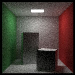
レンダリングされる画像を図 2.23 に示す。

インスタンス

普通コーネルボックスには二つの立方体があって、どちらも壁に対して角度が付いている。まず六個の長方形を使って辺が軸に平行な直方体を作ろう。

class box: public hittable  {
public:
  box() {}
  box(const point3& p0, const point3& p1, shared_ptr<material> ptr);

  virtual bool hit(const ray& r, double t0, double t1, hit_record& rec) const;

  virtual bool bounding_box(double t0, double t1, aabb& output_box) const {
    output_box = aabb(box_min, box_max);
    return true;
  }

public:
  point3 box_min;
  point3 box_max;
  hittable_list sides;
};

box::box(const point3& p0, const point3& p1, shared_ptr<material> ptr) {
  box_min = p0;
  box_max = p1;

  sides.add(make_shared<xy_rect>(p0.x(), p1.x(), p0.y(), p1.y(), p1.z(), ptr));
  sides.add(make_shared<xy_rect>(p0.x(), p1.x(), p0.y(), p1.y(), p0.z(), ptr));

  sides.add(make_shared<xz_rect>(p0.x(), p1.x(), p0.z(), p1.z(), p1.y(), ptr));
  sides.add(make_shared<xz_rect>(p0.x(), p1.x(), p0.z(), p1.z(), p0.y(), ptr));

  sides.add(make_shared<yz_rect>(p0.y(), p1.y(), p0.z(), p1.z(), p1.x(), ptr));
  sides.add(make_shared<yz_rect>(p0.y(), p1.y(), p0.z(), p1.z(), p0.x(), ptr));
}

bool box::hit(const ray& r, double t0, double t1, hit_record& rec) const {
  return sides.hit(r, t0, t1, rec);
}

リスト 2.58 [box.h] box クラス

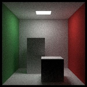
続いてシーンに二つの直方体を追加する。まだ角度は付いていない。

objects.add(make_shared<box>(point3(130, 0, 65), point3(295, 165, 230), white));
objects.add(make_shared<box>(point3(265, 0, 295), point3(430, 330, 460), white));

リスト 2.59 [main.cc] box をシーンに追加する

次の画像が得られる:

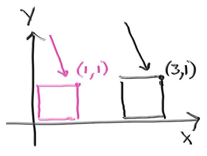
さらに立方体を回転させれば真のコーネルボックスとなる。レイトレーシングではオブジェクトの回転や移動を実装するのにインスタンス (instance) という考え方を使うことが多い。インスタンスとはある幾何形状を移動あるいは回転させて得られる幾何形状のことである。レイトレーシングでは物体の移動がレイの移動で済むので、インスタンスの取り扱いが非常に簡単になる。例えば下図のピンクの四角を \(x\) 軸正方向に \(2\) だけ移動したインスタンスと黒いレイの衝突を判定したいとする。このとき実際に移動させた黒い四角を使うこともできるし、\(x\) 軸正方向に \(-2\) だけ移動させたピンク色のレイを使うこともできる。レイトレーシングで使うのは後者である。

インスタンスの移動

物体を動かすと考えても座標を変えると考えてもどちらでも構わない。hittable を動かしてできる移動 (translation) インスタンスのコードは次の通りである:

class translate : public hittable {
public:
  translate(shared_ptr<hittable> p, const vec3& displacement)
    : ptr(p), offset(displacement) {}

  virtual bool hit(
    const ray& r, double t_min, double t_max, hit_record& rec
  ) const;
  virtual bool bounding_box(double t0, double t1, aabb& output_box) const;

public:
  shared_ptr<hittable> ptr;
  vec3 offset;
};

bool translate::hit(
  const ray& r, double t_min, double t_max, hit_record& rec
) const {
  ray moved_r(r.origin() - offset, r.direction(), r.time());
  if (!ptr->hit(moved_r, t_min, t_max, rec))
    return false;

  rec.p += offset;
  rec.set_face_normal(moved_r, rec.normal);

  return true;
}

bool translate::bounding_box(double t0, double t1, aabb& output_box) const {
  if (!ptr->bounding_box(t0, t1, output_box))
    return false;

  output_box = aabb(
    output_box.min() + offset,
    output_box.max() + offset);

  return true;
}

リスト 2.60 [hittable.h] translation クラス

インスタンスの回転

回転 (rotation) を理解して公式を導出するのは移動ほど簡単ではない。グラフィックスでは \(x\), \(y\), \(z\) 軸周りの回転を順に考えるのが一般的である。この三つの回転はある意味で「軸に平行」となる。最初に \(z\) 軸周りの回転を考える。\(x\) 座標と \(y\) 座標だけが変化し、その変化量には \(z\) 座標が関係しない。

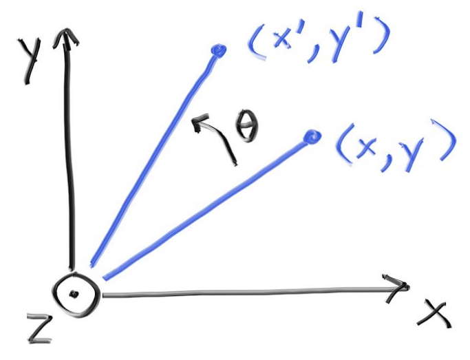
この回転を表す式の導出には三角関数の基本的な性質を用いる。ここでは説明しないが、グラフィックスの教科書あるいは講義ノートに必ず載っている。\(z\) 軸周りの反時計回りの回転を表す式は多少複雑で、次のようになる: \[ \begin{aligned} x' & = \cos \theta \cdot x - \sin \theta \cdot y \\ y' & = \sin \theta \cdot x + \cos \theta \cdot y \end{aligned} \] この式は任意の \(\theta\) で成り立ち、場合分けが必要ないのが素晴らしい。この逆変換は幾何学的に逆の操作つまり \(-\theta\) の回転であり、\(\cos \theta = \cos(-\theta)\) と \(\sin(-\theta) = -\sin \theta\) を使えば簡単に求まる。

同様に \(y\) 軸周りの回転 (コーネルボックスで使う回転) は \[ \begin{aligned} x' & = \hphantom{-} \cos \theta \cdot x + \sin \theta \cdot z \\ z' & = -\sin \theta \cdot x + \cos \theta \cdot z \end{aligned} \] であり、\(x\) 軸周りの回転は \[ \begin{aligned} y' & = \cos \theta \cdot y - \sin \theta \cdot z \\ z' & = \sin \theta \cdot y + \cos \theta \cdot z \end{aligned} \] となる。

移動の場合と異なり、回転では曲面の法線も変化する。そのため衝突を検出したときに法線の方向を変更しなければならないが、幸い回転では法線にも同じ式を利用できる。ただし拡大を伴う場合には法線の変換が複雑になるので注意がいる。https://in1weekend.blogspot.com/ に参考ページを載せておいた。

\(y\) 軸周りの回転インスタンスのクラスは次の通りである:

class rotate_y : public hittable {
public:
  rotate_y(shared_ptr<hittable> p, double angle);
  virtual bool hit(const ray& r, double t_min, double t_max, hit_record& rec) const;

  virtual bool bounding_box(double t0, double t1, aabb& output_box) const {
    output_box = bbox;
    return hasbox;
  }

public:
  shared_ptr<hittable> ptr;
  double sin_theta;
  double cos_theta;
  bool hasbox;
  aabb bbox;
};

リスト 2.61 [hittable.h] rotate_y クラス

コンストラクタを示す:

rotate_y::rotate_y(shared_ptr<hittable> p, double angle) : ptr(p) {
  auto radians = degrees_to_radians(angle);
  sin_theta = sin(radians);
  cos_theta = cos(radians);
  hasbox = ptr->bounding_box(0, 1, bbox);
  point3 min( infinity,  infinity,  infinity);
  point3 max(-infinity, -infinity, -infinity);

  for (int i = 0; i < 2; i++) {
    for (int j = 0; j < 2; j++) {
      for (int k = 0; k < 2; k++) {
        auto x = i*bbox.max().x() + (1-i)*bbox.min().x();
        auto y = j*bbox.max().y() + (1-j)*bbox.min().y();
        auto z = k*bbox.max().z() + (1-k)*bbox.min().z();
        auto newx =  cos_theta*x + sin_theta*z;
        auto newz = -sin_theta*x + cos_theta*z;

        vec3 tester(newx, y, newz);

        for (int c = 0; c < 3; c++) {
          min[c] = fmin(min[c], tester[c]);
          max[c] = fmax(max[c], tester[c]);
        }
      }
    }
  }

  bbox = aabb(min, max);
}

リスト 2.62 [hittable.h] rotate_y のコンストラクタ

hit 関数は次のようにできる:

bool rotate_y::hit(
  const ray& r, double t_min, double t_max, hit_record& rec
) const {
  auto origin = r.origin();
  auto direction = r.direction();
  origin[0] = cos_theta*r.origin()[0] - sin_theta*r.origin()[2];
  origin[2] = sin_theta*r.origin()[0] + cos_theta*r.origin()[2];
  direction[0] = cos_theta*r.direction()[0] - sin_theta*r.direction()[2];
  direction[2] = sin_theta*r.direction()[0] + cos_theta*r.direction()[2];

  ray rotated_r(origin, direction, r.time());

  if (!ptr->hit(rotated_r, t_min, t_max, rec))
    return false;

  auto p = rec.p;
  auto normal = rec.normal;

  p[0] =  cos_theta*rec.p[0] + sin_theta*rec.p[2];
  p[2] = -sin_theta*rec.p[0] + cos_theta*rec.p[2];

  normal[0] =  cos_theta*rec.normal[0] + sin_theta*rec.normal[2];
  normal[2] = -sin_theta*rec.normal[0] + cos_theta*rec.normal[2];

  rec.p = p;
  rec.set_face_normal(rotated_r, normal);

  return true;
}

リスト 2.63 [hittable.h] rotate_y::hit 関数

コーネルボックスを変更しよう:

shared_ptr<hittable> box1 =
  make_shared<box>(point3(0, 0, 0), point3(165, 330, 165), white);
box1 = make_shared<rotate_y>(box1,  15);
box1 = make_shared<translate>(box1, vec3(265,0,295));
objects.add(box1);

shared_ptr<hittable> box2 =
  make_shared<box>(point3(0,0,0), point3(165,165,165), white);
box2 = make_shared<rotate_y>(box2, -18);
box2 = make_shared<translate>(box2, vec3(130,0,65));
objects.add(box2);

リスト 2.64 [main.cc] 直方体を \(y\) 軸周りに回転させたコーネルボックス

次の画像が得られる:

ボリュームレンダリング

レイトレーサーにぜひ追加したいのがフォグ (煙・霧) だ。これはボリューム (volume) あるいは関与媒質 (participating media) とも呼ばれる。またオブジェクト内部の濃い霧として表面下散乱 (subsuraface scattering) も追加しておきたい。こういった概念は物体の表面と大きく異なる代物なので、普通に実装するとソフトウェアのアーキテクチャがうんと複雑になる。しかしここでは、ボリュームをランダムな表面とみなすテクニックが使える。つまり煙が存在する領域を確率的に衝突する表面を持った物体で置き換えるのである。どういうことかはコードを見ればより理解できるだろう。

定数密度媒質

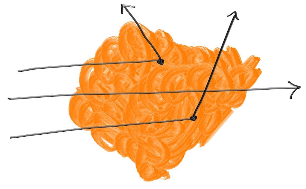
ここでは密度が定数の媒質だけを考える。この媒質中を進むレイは途中で散乱する可能性もあるし、散乱せずに突き抜ける可能性もある (下図)。媒質の透明度が高いと (煙が薄いと) 図中央のような突き抜けるレイが増える。またレイが媒質中を通る長さもレイが散乱する可能性に影響する。

媒質中を進むレイは任意の点で散乱する可能性があり、媒質が濃いとそれだけ散乱しやすくなる。レイが小さい距離 \(\Delta L\) を進むときに散乱する確率は \[ {\footnotesize \text{散乱する確率}} = C \cdot \Delta L \] と表せる。ここで \(C\) は媒質の光学的密度に比例する。この微分方程式を全ての点で考えることで、乱数を散乱が起こる距離に結び付けることができる ⁵。この距離が媒質の外側ならレイは媒質と「衝突」しない。密度が定数の媒質に対しては \(C\) と境界の情報があればこの計算が行える。境界には別の hittable を使うとすれば、次のクラスが書ける:

class constant_medium : public hittable {
public:
  constant_medium(shared_ptr<hittable> b, double d, shared_ptr<texture> a)
    : boundary(b), neg_inv_density(-1/d) {
    phase_function = make_shared<isotropic>(a);
  }

  virtual bool hit(
    const ray& r, double t_min, double t_max, hit_record& rec
  ) const;

  virtual bool bounding_box(double t0, double t1, aabb& output_box) const {
    return boundary->bounding_box(t0, t1, output_box);
  }

public:
  shared_ptr<hittable> boundary;
  shared_ptr<material> phase_function;
  double neg_inv_density;
};

リスト 2.65 [constant_medium.h] constant_medium クラス

等方性 (isotropic) テクスチャの scatter 関数は方向を一様ランダムに選ぶ:

class isotropic : public material {
public:
  isotropic(shared_ptr<texture> a) : albedo(a) {}

  virtual bool scatter(
    const ray& r_in,
    const hit_record& rec,
    color& attenuation,
    ray& scattered
  ) const {
    scattered = ray(rec.p, random_in_unit_sphere(), r_in.time());
    attenuation = albedo->value(rec.u, rec.v, rec.p);
    return true;
  }

public:
  shared_ptr<texture> albedo;
};

リスト 2.66 [material.h] isotropic クラス

そして hit 関数はこれだ:

bool constant_medium::hit(
  const ray& r, double t_min, double t_max, hit_record& rec
) const {
  // デバッグ中には低い確率でサンプルの様子を出力する。
  // enableDebug を true にすると有効になる。
  const bool enableDebug = false;
  const bool debugging = enableDebug && random_double() < 0.00001;

  hit_record rec1, rec2;

  if (!boundary->hit(r, -infinity, infinity, rec1))
    return false;

  if (!boundary->hit(r, rec1.t+0.0001, infinity, rec2))
    return false;

  if (debugging) std::cerr << "\nt0=" << rec1.t << ", t1=" << rec2.t << '\n';

  if (rec1.t < t_min) rec1.t = t_min;
  if (rec2.t > t_max) rec2.t = t_max;

  if (rec1.t >= rec2.t)
    return false;

  if (rec1.t < 0)
    rec1.t = 0;

  const auto ray_length = r.direction().length();
  const auto distance_inside_boundary = (rec2.t - rec1.t) * ray_length;
  const auto hit_distance = neg_inv_density * log(random_double());

  if (hit_distance > distance_inside_boundary)
    return false;

  rec.t = rec1.t + hit_distance / ray_length;
  rec.p = r.at(rec.t);

  if (debugging) {
    std::cerr << "hit_distance = " <<  hit_distance << '\n'
          << "rec.t = " <<  rec.t << '\n'
          << "rec.p = " <<  rec.p << '\n';
  }

  rec.normal = vec3(1,0,0); // どんな値でもよい
  rec.front_face = true;    // 同じくどんな値でもよい
  rec.mat_ptr = phase_function;

  return true;
}

リスト 2.67 [constant_medium.h] constant_medium::hit 関数

この関数はレイの始点が媒質の中にある場合にも正しい必要があるので、境界が関係する処理は慎重に行う必要がある。雲の中ではレイが何度も跳ね返るので、視点が媒質の中にあるレイは珍しいものではない。

このコードでは一度媒質に入ってから出たレイは二度と媒質に入らないことが仮定されている。言い換えると、境界の形状は凸である必要がある。この実装は直方体や球といった境界に対しては正しく動くが、穴を含むトーラスのような境界ではうまく動かない。任意の形状を扱える実装も可能だが、これは読者への練習問題とする。

煙がかった直方体のレンダリング

コーネルボックスの直方体を煙と霧 (暗いボリュームと明るいボリューム) に変えて、収束を速めるためにライトを大きく (さらに明るさで白飛びしないように暗く) する:

hittable_list cornell_smoke() {
  hittable_list objects;

  auto red   = make_shared<lambertian>(make_shared<solid_color>(.65, .05, .05));
  auto white = make_shared<lambertian>(make_shared<solid_color>(.73, .73, .73));
  auto green = make_shared<lambertian>(make_shared<solid_color>(.12, .45, .15));
  auto light = make_shared<diffuse_light>(make_shared<solid_color>(7, 7, 7));

  objects.add(make_shared<yz_rect>(0, 555, 0, 555, 555, green));
  objects.add(make_shared<yz_rect>(0, 555, 0, 555, 0, red));
  objects.add(make_shared<xz_rect>(113, 443, 127, 432, 554, light));
  objects.add(make_shared<xz_rect>(0, 555, 0, 555, 555, white));
  objects.add(make_shared<xz_rect>(0, 555, 0, 555, 0, white));
  objects.add(make_shared<xy_rect>(0, 555, 0, 555, 555, white));

  shared_ptr<hittable> box1 =
    make_shared<box>(point3(0,0,0), point3(165,330,165), white);
  box1 = make_shared<rotate_y>(box1,  15);
  box1 = make_shared<translate>(box1, vec3(265,0,295));

  shared_ptr<hittable> box2 =
    make_shared<box>(point3(0,0,0), point3(165,165,165), white);
  box2 = make_shared<rotate_y>(box2, -18);
  box2 = make_shared<translate>(box2, vec3(130,0,65));

  objects.add(
    make_shared<constant_medium>(box1, 0.01, make_shared<solid_color>(0,0,0))
  );
  objects.add(
    make_shared<constant_medium>(box2, 0.01, make_shared<solid_color>(1,1,1))
  );

  return objects;
}

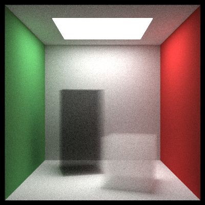
リスト 2.68 [main.cc] 煙を使ったコーネルボックス

次の画像が得られる:

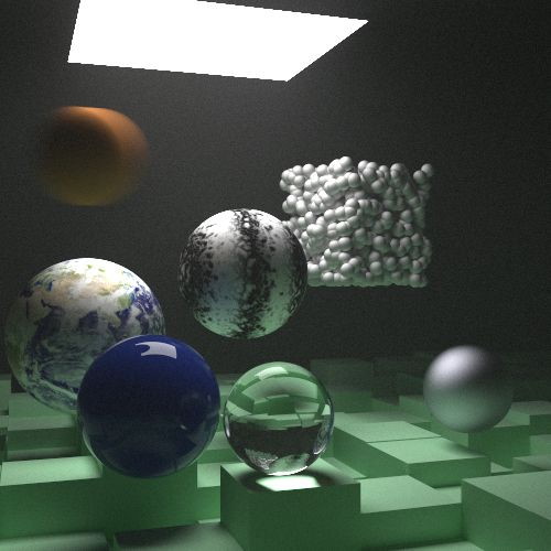
新しい機能を全て使ったシーン

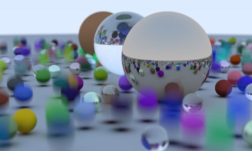
全ての機能を一つのシーンにまとめよう。さらに全体に広がる薄い霧と表面下反射 (クリアコート層) を持つ青い球も追加する (表面下反射は直接実装していないが、拡散マテリアルを誘電体マテリアルで包んだものが表面下反射を起こすマテリアルに等しい)。このレンダラの最大の制限はシャドウレイがないことだが、これと引き換えに集光模様と表面下散乱が手に入っている。これは諸刃の剣の設計判断だ。

hittable_list final_scene() {
  hittable_list boxes1;
  auto ground =
    make_shared<lambertian>(make_shared<solid_color>(0.48, 0.83, 0.53));

  const int boxes_per_side = 20;
  for (int i = 0; i < boxes_per_side; i++) {
    for (int j = 0; j < boxes_per_side; j++) {
      auto w = 100.0;
      auto x0 = -1000.0 + i*w;
      auto z0 = -1000.0 + j*w;
      auto y0 = 0.0;
      auto x1 = x0 + w;
      auto y1 = random_double(1,101);
      auto z1 = z0 + w;

      boxes1.add(make_shared<box>(point3(x0,y0,z0), point3(x1,y1,z1), ground));
    }
  }

  hittable_list objects;

  objects.add(make_shared<bvh_node>(boxes1, 0, 1));

  auto light = make_shared<diffuse_light>(make_shared<solid_color>(7, 7, 7));
  objects.add(make_shared<xz_rect>(123, 423, 147, 412, 554, light));

  auto center1 = point3(400, 400, 200);
  auto center2 = center1 + vec3(30,0,0);
  auto moving_sphere_material =
    make_shared<lambertian>(make_shared<solid_color>(0.7, 0.3, 0.1));
  objects.add(make_shared<moving_sphere>(
    center1, center2, 0, 1, 50, moving_sphere_material));

  objects.add(make_shared<sphere>(
    point3(260, 150, 45), 50, make_shared<dielectric>(1.5)));
  objects.add(make_shared<sphere>(
    point3(0, 150, 145), 50, make_shared<metal>(color(0.8, 0.8, 0.9), 10.0)));

  auto boundary = make_shared<sphere>(
    point3(360,150,145), 70, make_shared<dielectric>(1.5));
  objects.add(boundary);
  objects.add(make_shared<constant_medium>(
    boundary, 0.2, make_shared<solid_color>(0.2, 0.4, 0.9)));
  boundary = make_shared<sphere>(
    point3(0, 0, 0), 5000, make_shared<dielectric>(1.5));
  objects.add(make_shared<constant_medium>(
    boundary, .0001, make_shared<solid_color>(1,1,1)));

  auto emat = make_shared<lambertian>(
    make_shared<image_texture>("earthmap.jpg"));
  objects.add(make_shared<sphere>(point3(400,200,400), 100, emat));
  auto pertext = make_shared<noise_texture>(0.1);
  objects.add(make_shared<sphere>(
    point3(220,280,300), 80, make_shared<lambertian>(pertext)));

  hittable_list boxes2;
  auto white = make_shared<lambertian>(make_shared<solid_color>(.73, .73, .73));
  int ns = 1000;
  for (int j = 0; j < ns; j++) {
    boxes2.add(make_shared<sphere>(point3::random(0,165), 10, white));
  }

  objects.add(make_shared<translate>(
    make_shared<rotate_y>(
      make_shared<bvh_node>(boxes2, 0.0, 1.0), 15),
      vec3(-100,270,395)
    )
  );

  return objects;
}

リスト 2.69 [main.cc] 最後のシーン

\(1\) ピクセルごとに \(10{,}000\) レイを放てば次の画像が得られる:

さぁクールな画像を自分で作ってみよ！発展的な文献やここで紹介しなかった機能は https://in1weekend.blogspot.com/ にまとめてある。質問やコメント、クールな画像は ptrshrl@gmail.com まで送ってほしい。

謝辞

初稿

Dave Hart
Jean Buckley

ウェブリリース

Berna Kabadayı
Lorenzo Mancini
Lori Whippler Hollasch
Ronald Wotzlaw

訂正・改善

Aaryaman Vasishta
Andrew Kensler
Apoorva Joshi
Aras Pranckevičius
Becker
Ben Kerl
Benjamin Summerton
Bennett Hardwick
Dan Drummond
David Chambers
David Hart
Eric Haines
Fabio Sancinetti
Filipe Scur
Frank He
Gerrit Wessendorf
Grue Debry
Ingo Wald
Jason Stone
Jean Buckley
Joey Cho
Lorenzo Mancini
Marcus Ottosson
Matthew Heimlich
Nakata Daisuke
Paul Melis
Phil Cristensen
Ronald Wotzlaw
Shaun P. Lee
Tatsuya Ogawa
Thiago Ize
Vahan Sosoyan
ZeHao Chen

ツール

図の作成に利用した Limnu のチームに感謝する。

このシリーズ⁶は Morgan McGuire による素晴らしい無料ライブラリ Markdeep を使って執筆された。ブラウザからソースを閲覧すれば、どのように書かれたかを確認できる。

訳注: 英語版のタイトルは第一巻が "Ray Tracing In One Weekend" で、第二巻が "Ray Tracing: The Next Week" である。^[return]
訳注: 関数 \(f(n)\) が劣線形 (sublinear) であるとは、\(n \to \infty\) で \(f(n)/n \to 0\) となることを言う。^[return]
訳注: 「スラブ (slab)」は金属や木材の薄い板を意味する。^[return]
出典: Wikipedia Commons (パブリックドメイン)^[return]
訳注: レイが媒質中を散乱せずに \(L = n\Delta L\) だけ進み、その直後に散乱する確率を \(p(L)\) とする。このとき \(p(L) \propto \left(1 - C\Delta L\right)^{n} = \left(1 - C\Delta L\right)^{\frac{L}{\Delta L}}\) が成り立ち、\(\Delta L \to 0\) つまり \(n \to \infty\) のとき \(p(L) \to k e^{-CL}\) となる (\(k\) は定数)。確率を全区間で積分すれば \(1\) だから \[\int_{0}^{\infty} p(L) \, dL = \int_{0}^{\infty} ke^{-CL} \, dL = \frac{k}{C} = 1\] であり、\(k = C\) が分かる。\([0,1]\) の一様乱数 \(r\) に対して \[r = \int_{0}^{x} p(x)\,dx = \int_{0}^{x} Ce^{-Cx} \,dx = 1 - e^{-Cx} \] が成り立つとき \(x\) の確率密度関数は \(p(x)\) となる。よってこの等式を \(x\) について解いた \[x = -\frac{1}{C}\log(1 - r)\] という関係を使えばレイが散乱するまでの「ランダムな」長さを計算できる。^[return]
訳注: 英語版のこと。^[return]

週末レイトレーシング 第二週 (翻訳)

はじめに

モーションブラー

時空間レイトレーシング入門

モーションブラーをシミュレートするカメラ

運動する球の追加

レイが衝突したときの時間の伝播

まとめ

包含立体階層

基本的なアイデア

包含立体階層

軸平行包含直方体

AABB を使ったレイの衝突判定

AABB の衝突判定の最適化

AABB の構築

オブジェクトリストの AABB の計算

BVH を表すクラス

BVH の分割

AABB の比較関数

最初のテクスチャクラス: 定数テクスチャ

球のテクスチャ座標

縞模様テクスチャ

縞模様テクスチャを使ったシーンのレンダリング

パーリンノイズ

乱数のブロック

ノイズのスムージング

エルミート補間によるノイズの改善

周波数の調整

格子点にランダムなベクトルを配置する

乱流ノイズ

位相の調整

画像のテクスチャマッピング

画像データの読み込み

画像テクスチャを使う

長方形とライト

発光マテリアル

背景を黒くする

長方形オブジェクト

オブジェクトを光源にする

その他の軸に垂直な長方形

空のコーネルボックスの作成

インスタンス

インスタンスの移動

インスタンスの回転

ボリュームレンダリング

定数密度媒質

煙がかった直方体のレンダリング

新しい機能を全て使ったシーン

謝辞

初稿

ウェブリリース

訂正・改善

ツール

週末レイトレーシング第二週 (翻訳)